createSurfaceMap <- function(df, var_name, legend_min, legend_max){
# additional: parameters
# model = try "Sph" (spherical), "Exp" (exponential) or "Gau" (Gaussian) to get the best variogram fit
MODEL <- "Exp"
# length.out Increase for a finer grid (slower), decrease for speed
LENGTH_OUT = 300
# bbox_ext = 0.1 Adjust padding around your data extent (in degrees)
#A nugget = 0 Set to a small positive value if data has measurement error
output <- tryCatch({
# get average value of var_name for 0-5 meters in df
df <- df %>%
filter(depth >= 0 & depth <= 5) %>%
group_by(station) %>%
summarise(
mean_value = mean(.data[[var_name]], na.rm = TRUE),
latitude = first(na.omit(latitude)),
longitude = first(na.omit(longitude)),
.groups = "drop"
)
librarian::shelf(
quiet = TRUE,
sp, gstat, ggplot2, viridis, raster, sf
)
# --- 1. Prepare spatial data ---
df_sp <- df
df_sp$latitude <- as.numeric(df_sp$latitude)
df_sp$longitude <- as.numeric(df_sp$longitude)
df_sp <- df_sp[!is.na(df_sp$mean_value) & !is.na(df_sp$latitude) & !is.na(df_sp$longitude), ]
coordinates(df_sp) <- ~longitude + latitude
proj4string(df_sp) <- CRS("+proj=longlat +datum=WGS84")
# --- 2. Create interpolation grid ---
bbox_ext <- 0.1
lon_range <- seq(bbox(df_sp)[1,1] - bbox_ext, bbox(df_sp)[1,2] + bbox_ext, length.out = LENGTH_OUT)
lat_range <- seq(bbox(df_sp)[2,1] - bbox_ext, bbox(df_sp)[2,2] + bbox_ext, length.out = LENGTH_OUT)
grid <- expand.grid(longitude = lon_range, latitude = lat_range)
coordinates(grid) <- ~longitude + latitude
proj4string(grid) <- CRS("+proj=longlat +datum=WGS84")
gridded(grid) <- TRUE
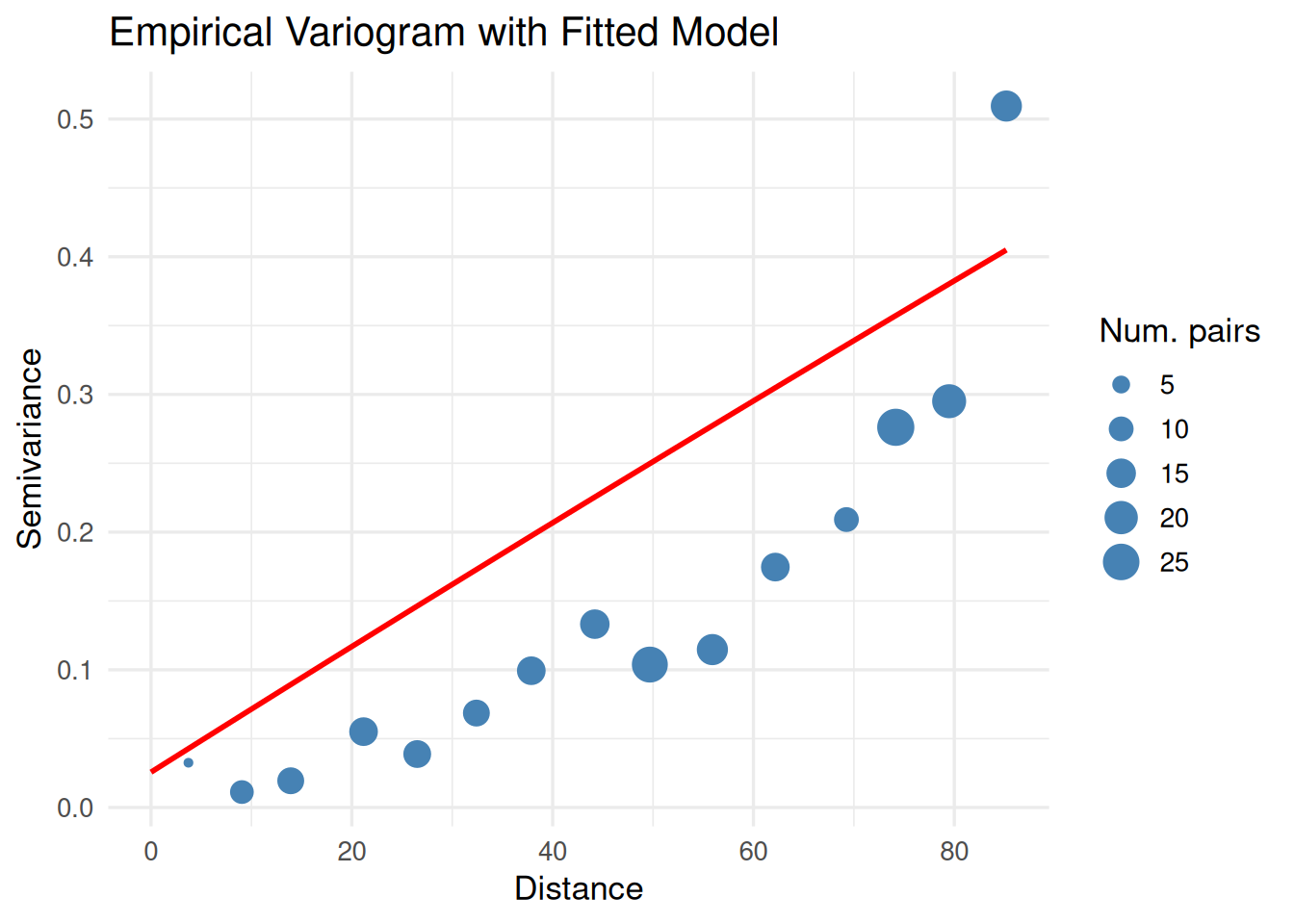
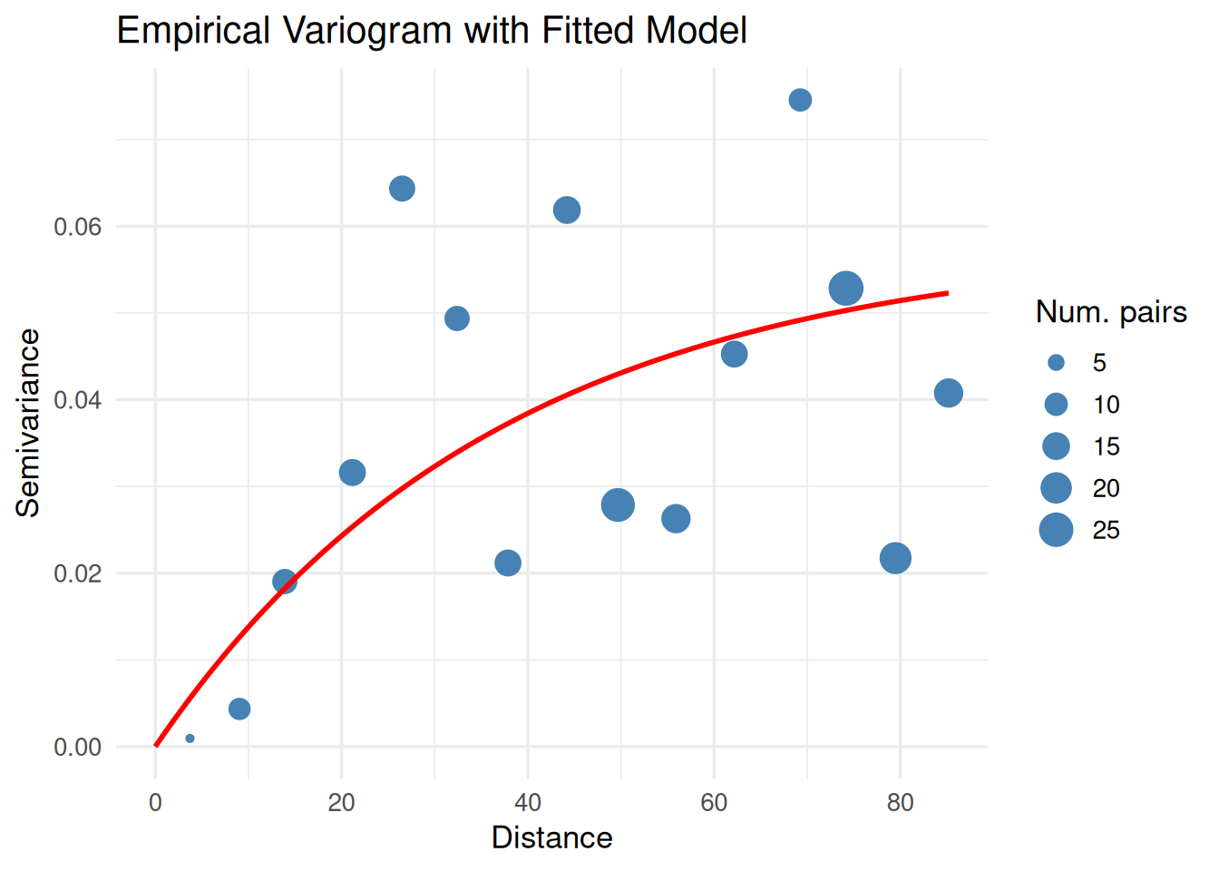
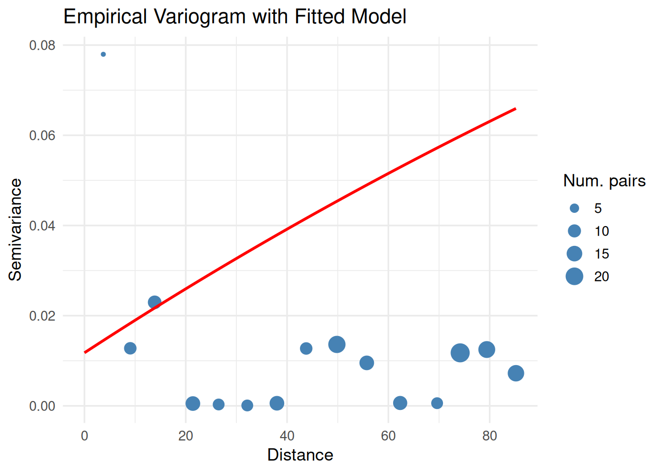
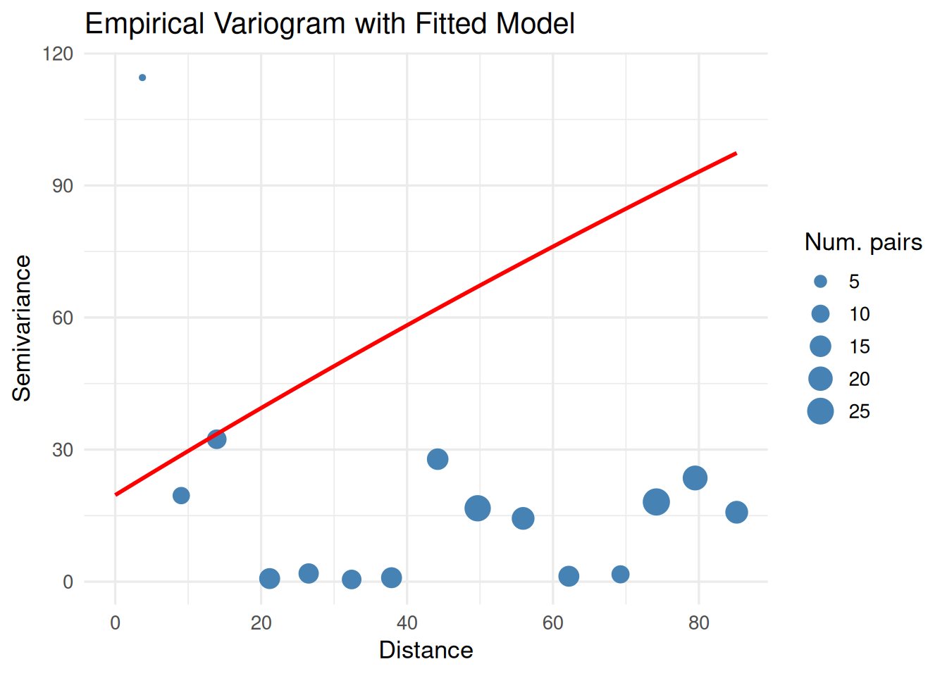
# --- 3. Fit variogram ---
vgm_emp <- variogram(mean_value ~ 1, data = df_sp)
vgm_fit <- fit.variogram(vgm_emp, model = vgm(
psill = max(vgm_emp$gamma),
model = MODEL,
range = max(vgm_emp$dist) / 2,
nugget = min(vgm_emp$gamma)
))
vgm_line <- variogramLine(vgm_fit, maxdist = max(vgm_emp$dist))
print(
ggplot() +
geom_point(data = vgm_emp, aes(x = dist, y = gamma, size = np), color = "steelblue") +
geom_line(data = vgm_line, aes(x = dist, y = gamma), color = "red", linewidth = 1) +
labs(title = "Empirical Variogram with Fitted Model",
x = "Distance", y = "Semivariance", size = "Num. pairs") +
theme_minimal(base_size = 13)
)
# --- 4. Perform Ordinary Kriging ---
krig_result <- suppressWarnings(krige(
mean_value ~ 1,
locations = df_sp,
newdata = grid,
model = vgm_fit
))
# --- 5. Convert to data frame and clip to convex hull ---
krig_df <- as.data.frame(krig_result)
names(krig_df)[names(krig_df) == "var1.pred"] <- "predicted"
names(krig_df)[names(krig_df) == "var1.var"] <- "variance"
# Build convex hull from sample points
pts_sf <- st_as_sf(df, coords = c("longitude", "latitude"), crs = 4326)
hull_sf <- st_convex_hull(st_union(pts_sf))
# Clip kriged grid to hull
krig_sf <- st_as_sf(krig_df, coords = c("longitude", "latitude"), crs = 4326)
krig_clipped <- st_filter(krig_sf, hull_sf)
krig_df <- cbind(st_drop_geometry(krig_clipped), st_coordinates(krig_clipped))
names(krig_df)[names(krig_df) == "X"] <- "longitude"
names(krig_df)[names(krig_df) == "Y"] <- "latitude"
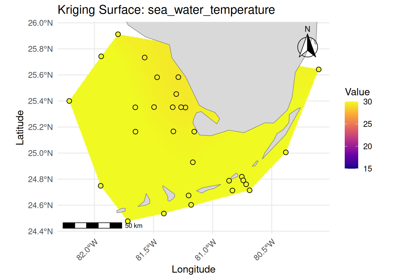
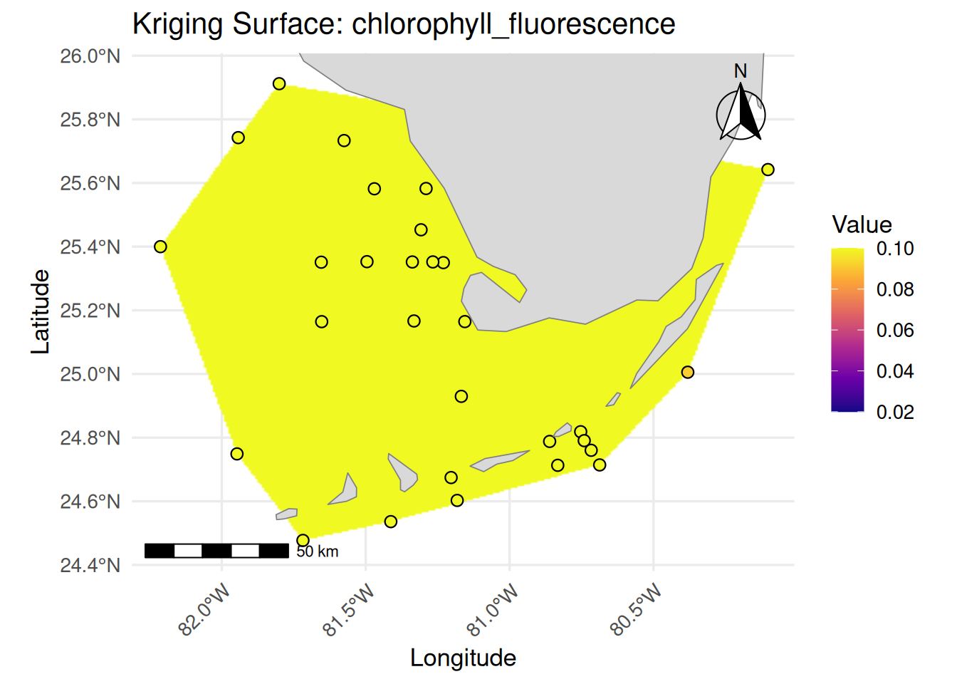
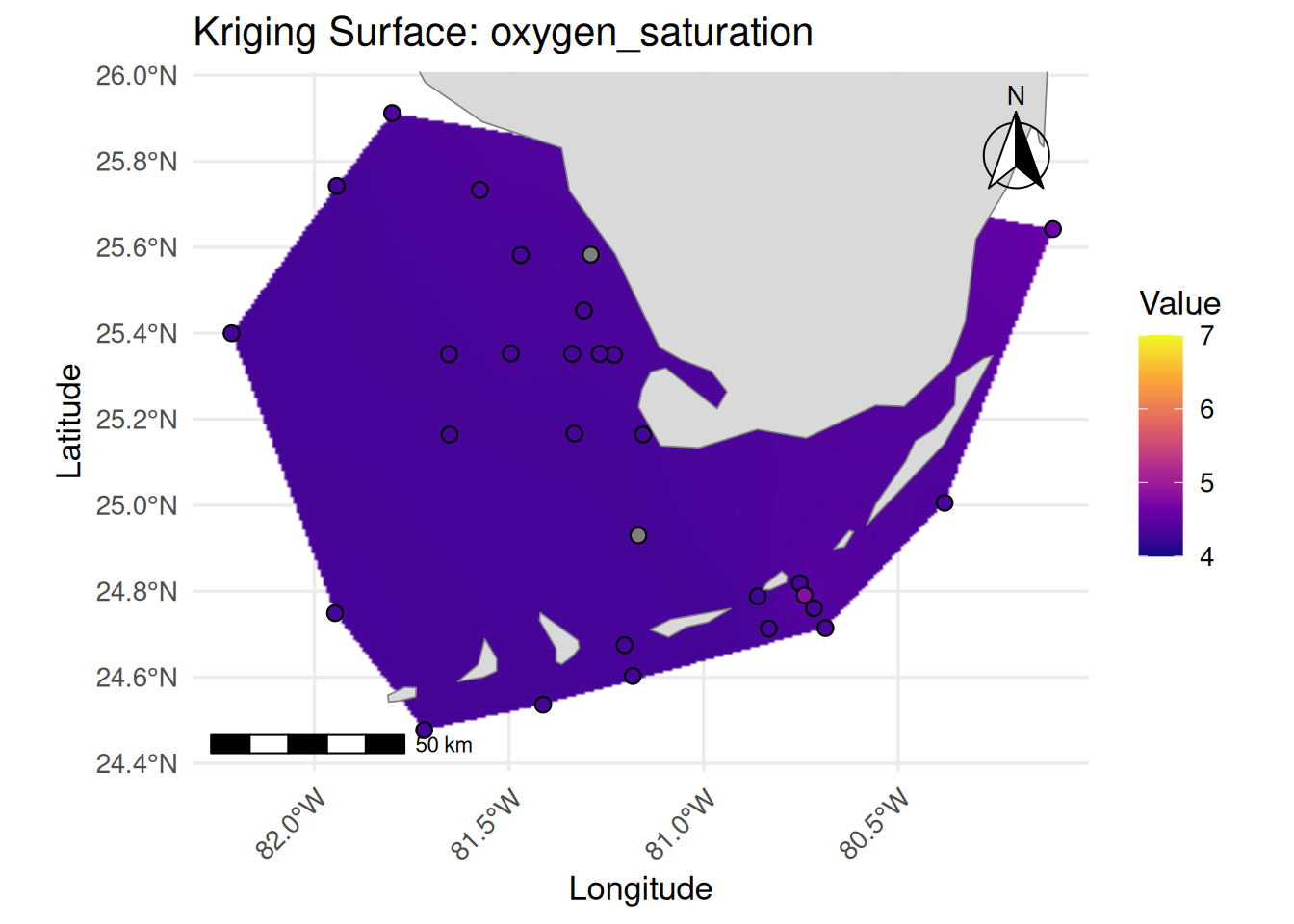
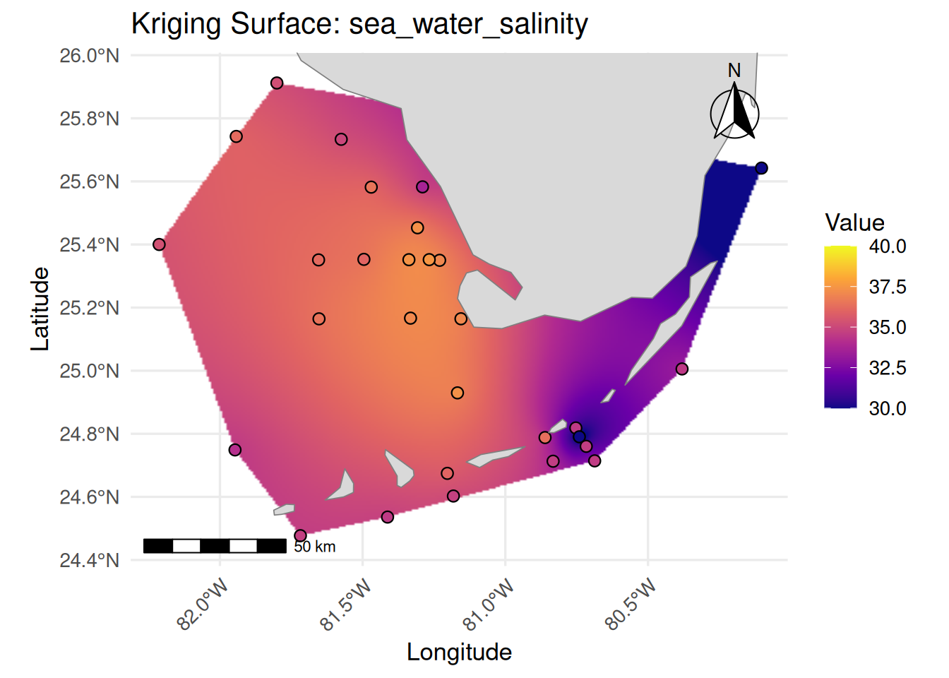
# --- 6. Plot surface map ---
librarian::shelf(quiet = TRUE, ggplot2, viridis, sf, ggspatial, rnaturalearth, rnaturalearthdata)
# --- Basemap ---
world <- ne_countries(scale = "medium", returnclass = "sf")
print(
ggplot() +
# Kriged surface
geom_raster(data = krig_df, aes(x = longitude, y = latitude, fill = predicted), interpolate = TRUE) +
geom_point(data = df, aes(x = longitude, y = latitude, fill = mean_value),
shape = 21, color = "black", size = 2.5) +
scale_fill_viridis_c(
option = "plasma",
name = "Value",
limits = c(legend_min, legend_max),
oob = scales::squish
) +
# Basemap
geom_sf(data = world, fill = "gray85", color = "gray50", linewidth = 0.3) +
# Colorscale with hardcoded limits
scale_fill_viridis_c(
option = "plasma",
name = "Value",
limits = c(legend_min, legend_max),
oob = scales::squish # squish values outside limits into the color range
) +
# Zoom to data extent with a small buffer
coord_sf(
xlim = c(min(krig_df$longitude) - 0.1, max(krig_df$longitude) + 0.1),
ylim = c(min(krig_df$latitude) - 0.1, max(krig_df$latitude) + 0.1),
expand = FALSE
) +
annotation_scale(location = "bl") +
annotation_north_arrow(location = "tr", style = north_arrow_fancy_orienteering()) +
labs(
title = paste("Kriging Surface:", var_name),
x = "Longitude", y = "Latitude"
) +
theme_minimal(base_size = 13) +
theme(axis.text.x = element_text(angle = 45, hjust = 1))
)
},
error = function(e) {
print(glue::glue("error generating surface map for {var_name}:"))
print(e)
})
}
createSurfaceMap(cruise_df, "sea_water_temperature", 15, 30)