seacar-check – FCRWQDC Ingest Reports

In 2026 management of this data is being transferred to SEACAR In this file we prepare a transformation of the dataset for SEACAR ingestion, and perform some checks.

The data here should align with standards described in SEACAR_Metadata_UnifiedWQ_ID10006.xlsx.

Code

librarian::shelf(
  dplyr,
  glue,
  here,
  tidyr
)

Code

library("here")
df_all <- read.csv(here("data/exports/allDataRaw.csv"))
source(here("R/dropNonStandardAnalytes.R"))
df <- dropNonStandardAnalytes(df_all)

source(here("R/mutateWINToSEACAR.R"))
df <- mutateWINToSEACAR(df)

# write SEACAR .csv
write.csv(df, here("data", "exports", "allDataSEACAR.csv"))

show percent of missing programID

library(dplyr)
library(scales)
# show percentage of missing or na rows 
# 1. Get the total number of rows for each program
total_counts <- df %>%
  count(ProgramName, name = "total_rows")

# 2. Get the number of NA rows for each program
na_counts <- df %>%
  filter(is.na(ProgramID)) %>%
  count(ProgramName, name = "missing_rows")

# 3. Combine total and NA counts, calculate percentage
percentage_table <- total_counts %>%
  left_join(na_counts, by = "ProgramName") %>%
  mutate(
    # If a program had no NAs, na_counts will be NA. Replace with 0.
    missing_rows = ifelse(is.na(missing_rows), 0, missing_rows),
    
    # Calculate the percentage
    percentage_raw = missing_rows / total_rows,
    
    # Format the percentage for clean table output
    percentage = scales::percent(percentage_raw, accuracy = 0.1)
  ) %>%
  
  # Select and order the columns for the final table
  select(ProgramName, missing_rows, total_rows, percentage) %>%
  
  # Sort by program name
  arrange(ProgramName)

# 4. Print the final data frame (which R displays as a table)
print(percentage_table)

           ProgramName missing_rows total_rows percentage
1            AOML_FBBB            0      49603       0.0%
2                 BBAP            0      10594       0.0%
3                 BBWW            0        910       0.0%
4              BROWARD            0      15142       0.0%
5       BROWARD_STORET            0      24290       0.0%
6                  DEP            0      99792       0.0%
7            DERM_BBWQ            0     144946       0.0%
8     DERM_BBWQ_STORET            0     442825       0.0%
9        FIU_Estuaries            0     412386       0.0%
10            FIU_WQMP            0      62621       0.0%
11 FIU_WQMP_HISTORICAL            0     484218       0.0%
12     FIU_WQMP_RECENT            0       4020       0.0%
13          MiamiBeach            0      27484       0.0%
14           PALMBEACH            0       7658       0.0%
15    PALMBEACH_STORET            0      13145       0.0%
16                SFER            0      84700       0.0%

show percent of missing SampleDate

library(dplyr)
library(scales)
# show percentage of missing or na rows 
# 1. Get the total number of rows for each program
total_counts <- df %>%
  count(ProgramName, name = "total_rows")

# 2. Get the number of NA rows for each program
na_counts <- df %>%
  filter(is.na(SampleDate)) %>%
  count(ProgramName, name = "missing_rows")

# 3. Combine total and NA counts, calculate percentage
percentage_table <- total_counts %>%
  left_join(na_counts, by = "ProgramName") %>%
  mutate(
    # If a program had no NAs, na_counts will be NA. Replace with 0.
    missing_rows = ifelse(is.na(missing_rows), 0, missing_rows),
    
    # Calculate the percentage
    percentage_raw = missing_rows / total_rows,
    
    # Format the percentage for clean table output
    percentage = scales::percent(percentage_raw, accuracy = 0.1)
  ) %>%
  
  # Select and order the columns for the final table
  select(ProgramName, missing_rows, total_rows, percentage) %>%
  
  # Sort by program name
  arrange(ProgramName)

# 4. Print the final data frame (which R displays as a table)
print(percentage_table)

           ProgramName missing_rows total_rows percentage
1            AOML_FBBB            0      49603       0.0%
2                 BBAP            0      10594       0.0%
3                 BBWW            0        910       0.0%
4              BROWARD            0      15142       0.0%
5       BROWARD_STORET            0      24290       0.0%
6                  DEP            0      99792       0.0%
7            DERM_BBWQ            0     144946       0.0%
8     DERM_BBWQ_STORET            0     442825       0.0%
9        FIU_Estuaries            0     412386       0.0%
10            FIU_WQMP            0      62621       0.0%
11 FIU_WQMP_HISTORICAL            0     484218       0.0%
12     FIU_WQMP_RECENT            0       4020       0.0%
13          MiamiBeach            0      27484       0.0%
14           PALMBEACH            0       7658       0.0%
15    PALMBEACH_STORET            0      13145       0.0%
16                SFER           20      84700       0.0%

show percent of missing ResultValue

library(dplyr)
library(scales)
# show percentage of missing or na rows 
# 1. Get the total number of rows for each program
total_counts <- df %>%
  count(ProgramName, name = "total_rows")

# 2. Get the number of NA rows for each program
na_counts <- df %>%
  filter(is.na(ResultValue)) %>%
  count(ProgramName, name = "missing_rows")

# 3. Combine total and NA counts, calculate percentage
percentage_table <- total_counts %>%
  left_join(na_counts, by = "ProgramName") %>%
  mutate(
    # If a program had no NAs, na_counts will be NA. Replace with 0.
    missing_rows = ifelse(is.na(missing_rows), 0, missing_rows),
    
    # Calculate the percentage
    percentage_raw = missing_rows / total_rows,
    
    # Format the percentage for clean table output
    percentage = scales::percent(percentage_raw, accuracy = 0.1)
  ) %>%
  
  # Select and order the columns for the final table
  select(ProgramName, missing_rows, total_rows, percentage) %>%
  
  # Sort by program name
  arrange(ProgramName)

# 4. Print the final data frame (which R displays as a table)
print(percentage_table)

           ProgramName missing_rows total_rows percentage
1            AOML_FBBB            1      49603       0.0%
2                 BBAP            3      10594       0.0%
3                 BBWW            0        910       0.0%
4              BROWARD            0      15142       0.0%
5       BROWARD_STORET         1410      24290       5.8%
6                  DEP            0      99792       0.0%
7            DERM_BBWQ           15     144946       0.0%
8     DERM_BBWQ_STORET         2850     442825       0.6%
9        FIU_Estuaries        21683     412386       5.3%
10            FIU_WQMP         2773      62621       4.4%
11 FIU_WQMP_HISTORICAL       121735     484218      25.1%
12     FIU_WQMP_RECENT          773       4020      19.2%
13          MiamiBeach          347      27484       1.3%
14           PALMBEACH           44       7658       0.6%
15    PALMBEACH_STORET          329      13145       2.5%
16                SFER        15367      84700      18.1%

show percent of missing coordinates

library(dplyr)
library(scales)
# show percentage of missing or na rows in df$Monitoring.Location.ID grouped by df$program
# 1. Get the total number of rows for each program
total_counts <- df %>%
  count(ProgramName, name = "total_rows")

# 2. Get the number of NA rows for each program
na_counts <- df %>%
  filter(is.na(OriginalLatitude) | is.na(OriginalLongitude)) %>%
  count(ProgramName, name = "missing_rows")

# 3. Combine total and NA counts, calculate percentage
percentage_table <- total_counts %>%
  left_join(na_counts, by = "ProgramName") %>%
  mutate(
    # If a program had no NAs, na_counts will be NA. Replace with 0.
    missing_rows = ifelse(is.na(missing_rows), 0, missing_rows),
    
    # Calculate the percentage
    percentage_raw = missing_rows / total_rows,
    
    # Format the percentage for clean table output
    percentage = scales::percent(percentage_raw, accuracy = 0.1)
  ) %>%
  
  # Select and order the columns for the final table
  select(ProgramName, missing_rows, total_rows, percentage) %>%
  
  # Sort by program name
  arrange(ProgramName)

# 4. Print the final data frame (which R displays as a table)
print(percentage_table)

           ProgramName missing_rows total_rows percentage
1            AOML_FBBB            0      49603       0.0%
2                 BBAP            0      10594       0.0%
3                 BBWW            0        910       0.0%
4              BROWARD            0      15142       0.0%
5       BROWARD_STORET        24290      24290     100.0%
6                  DEP            0      99792       0.0%
7            DERM_BBWQ            0     144946       0.0%
8     DERM_BBWQ_STORET       442825     442825     100.0%
9        FIU_Estuaries            0     412386       0.0%
10            FIU_WQMP            0      62621       0.0%
11 FIU_WQMP_HISTORICAL           54     484218       0.0%
12     FIU_WQMP_RECENT         4020       4020     100.0%
13          MiamiBeach         4443      27484      16.2%
14           PALMBEACH            0       7658       0.0%
15    PALMBEACH_STORET        13145      13145     100.0%
16                SFER           20      84700       0.0%

show percent of missing ProgramLocationID

library(dplyr)
library(scales)
# show percentage of missing or na rows 
# 1. Get the total number of rows for each program
total_counts <- df %>%
  count(ProgramName, name = "total_rows")

# 2. Get the number of NA rows for each program
na_counts <- df %>%
  filter(is.na(ProgramLocationID)) %>%
  count(ProgramName, name = "missing_rows")

# 3. Combine total and NA counts, calculate percentage
percentage_table <- total_counts %>%
  left_join(na_counts, by = "ProgramName") %>%
  mutate(
    # If a program had no NAs, na_counts will be NA. Replace with 0.
    missing_rows = ifelse(is.na(missing_rows), 0, missing_rows),
    
    # Calculate the percentage
    percentage_raw = missing_rows / total_rows,
    
    # Format the percentage for clean table output
    percentage = scales::percent(percentage_raw, accuracy = 0.1)
  ) %>%
  
  # Select and order the columns for the final table
  select(ProgramName, missing_rows, total_rows, percentage) %>%
  
  # Sort by program name
  arrange(ProgramName)

# 4. Print the final data frame (which R displays as a table)
print(percentage_table)

           ProgramName missing_rows total_rows percentage
1            AOML_FBBB            0      49603       0.0%
2                 BBAP            0      10594       0.0%
3                 BBWW            0        910       0.0%
4              BROWARD            0      15142       0.0%
5       BROWARD_STORET            0      24290       0.0%
6                  DEP            0      99792       0.0%
7            DERM_BBWQ            0     144946       0.0%
8     DERM_BBWQ_STORET            0     442825       0.0%
9        FIU_Estuaries            0     412386       0.0%
10            FIU_WQMP            0      62621       0.0%
11 FIU_WQMP_HISTORICAL            0     484218       0.0%
12     FIU_WQMP_RECENT            0       4020       0.0%
13          MiamiBeach            0      27484       0.0%
14           PALMBEACH            0       7658       0.0%
15    PALMBEACH_STORET            0      13145       0.0%
16                SFER           20      84700       0.0%

show percent of missing ParameterUnits

library(dplyr)
library(scales)
# show percentage of missing or na rows 
# 1. Get the total number of rows for each program
total_counts <- df %>%
  count(ProgramName, name = "total_rows")

# 2. Get the number of NA rows for each program
na_counts <- df %>%
  filter(is.na(ParameterUnits)) %>%
  count(ProgramName, name = "missing_rows")

# 3. Combine total and NA counts, calculate percentage
percentage_table <- total_counts %>%
  left_join(na_counts, by = "ProgramName") %>%
  mutate(
    # If a program had no NAs, na_counts will be NA. Replace with 0.
    missing_rows = ifelse(is.na(missing_rows), 0, missing_rows),
    
    # Calculate the percentage
    percentage_raw = missing_rows / total_rows,
    
    # Format the percentage for clean table output
    percentage = scales::percent(percentage_raw, accuracy = 0.1)
  ) %>%
  
  # Select and order the columns for the final table
  select(ProgramName, missing_rows, total_rows, percentage) %>%
  
  # Sort by program name
  arrange(ProgramName)

# 4. Print the final data frame (which R displays as a table)
print(percentage_table)

           ProgramName missing_rows total_rows percentage
1            AOML_FBBB            0      49603       0.0%
2                 BBAP            0      10594       0.0%
3                 BBWW            0        910       0.0%
4              BROWARD            0      15142       0.0%
5       BROWARD_STORET            0      24290       0.0%
6                  DEP            0      99792       0.0%
7            DERM_BBWQ            0     144946       0.0%
8     DERM_BBWQ_STORET            0     442825       0.0%
9        FIU_Estuaries            0     412386       0.0%
10            FIU_WQMP            0      62621       0.0%
11 FIU_WQMP_HISTORICAL            0     484218       0.0%
12     FIU_WQMP_RECENT         4020       4020     100.0%
13          MiamiBeach            0      27484       0.0%
14           PALMBEACH            0       7658       0.0%
15    PALMBEACH_STORET            0      13145       0.0%
16                SFER        84700      84700     100.0%

Code

#show table from df with a row for each unique of 
# (ProgramLocationID and ProgramName) with columns 
# programLocationID, ProgramName, and N_locations, 
# where N_locations is the number of unique OriginalLatitude and
# OriginalLongitude pairs for the programLocationID+ProgramName.

library(dplyr)

summary_table <- df %>%
  group_by(ProgramLocationID, ProgramName) %>%
  summarise(
    N_locations = n_distinct(paste(OriginalLatitude, OriginalLongitude)),
    .groups = "drop"
  ) %>%
  filter(N_locations > 1)

summary_table

# A tibble: 292 × 3
   ProgramLocationID ProgramName N_locations
   <chr>             <chr>             <int>
 1 1                 AOML_FBBB           133
 2 1                 SFER                 51
 3 10                AOML_FBBB           113
 4 10                SFER                 53
 5 11                AOML_FBBB           117
 6 11                SFER                 55
 7 12                AOML_FBBB           116
 8 12                SFER                 57
 9 13                AOML_FBBB           119
10 13                SFER                 54
# ℹ 282 more rows

Summary of column completeness

Code

skimr::skim(df)

Data summary
Name	df
Number of rows	1884334
Number of columns	35
_______________________
Column type frequency:
character	18
logical	1
numeric	16
________________________
Group variables	None

Variable type: character

skim_variable	n_missing	complete_rate	min	max	empty	n_unique	whitespace
Habitat	1519630	0.19	12	21	0	3	0
IndicatorName	1860383	0.01	9	13	0	3	0
ManagedAreaName	1860383	0.01	29	38	0	2	0
RelativeDepth	920543	0.51	0	7	17934	4	0
DetectionUnit	1882168	0.00	4	4	0	1	0
SEACAR_QAQCFlagCode	1860383	0.01	2	13	0	26	0
SEACAR_QAQC_Description	1860383	0.01	31	195	0	26	0
ExportVersion	1860383	0.01	23	23	0	3	0
Region	1810810	0.04	2	19	0	22	0
ProgramName	0	1.00	3	19	0	16	0
ParameterName	0	1.00	2	41	0	20	0
ParameterUnits	88720	0.95	0	10	14862	21	0
ProgramLocationID	20	1.00	1	25	0	2133	0
ActivityType	1542671	0.18	5	15	0	4	0
SampleDate	20	1.00	10	10	0	4591	0
ValueQualifier	1344472	0.29	0	4	221265	95	0
ResultComments	1543501	0.18	0	874	308298	756	10
SEACAR_EventID	1861293	0.01	36	36	0	2394	0

Variable type: logical

skim_variable	n_missing	complete_rate	mean	count
ValueQualifierSource	1884334	0	NaN	:

Variable type: numeric

skim_variable	n_missing	complete_rate	mean	sd	p0	p25	p50	p75	p100	hist
RowID	1861293	0.01	1009723.34	798651.12	486217.00	514368.00	534968.00	1551534.00	3870318.00	▇▂▁▁▁
ProgramID	0	1.00	2127.76	2351.03	3.00	297.00	509.00	4018.00	10013.00	▇▁▅▁▁
IndicatorID	1860383	0.01	6.73	0.63	6.00	6.00	7.00	7.00	8.00	▆▁▇▁▂
ParameterID	1860383	0.01	8.60	6.56	1.00	3.00	6.00	16.00	19.00	▇▃▁▂▅
AreaID	1860383	0.01	6.09	0.89	6.00	6.00	6.00	6.00	15.00	▇▁▁▁▁
Year	972961	0.48	2010.77	9.78	1989.48	2002.00	2011.00	2020.00	2024.00	▁▃▃▁▇
Month	972941	0.48	6.58	3.44	0.00	4.00	7.00	10.00	12.00	▅▅▇▆▇
TotalDepth_m	1884271	0.00	62.22	105.84	1.10	2.10	2.85	8.50	250.00	▇▁▁▁▂
MDL	1695992	0.10	0.06	0.49	0.00	0.00	0.01	0.08	50.50	▇▁▁▁▁
PQL	1695992	0.10	0.18	2.41	0.00	0.01	0.06	0.20	250.00	▇▁▁▁▁
Include	1860383	0.01	1.00	0.03	0.00	1.00	1.00	1.00	1.00	▁▁▁▁▇
MADup	1860383	0.01	1.00	0.00	1.00	1.00	1.00	1.00	1.00	▁▁▇▁▁
ResultValue	167330	0.91	10.82	385.27	-0.03	0.04	0.65	5.85	53465.00	▇▁▁▁▁
ActivityDepth_m	945466	0.50	6.51	20.98	0.00	0.50	3.00	8.46	3355.50	▇▁▁▁▁
OriginalLatitude	488743	0.74	25.36	0.63	24.38	24.85	25.29	25.78	28.78	▇▇▁▁▁
OriginalLongitude	488797	0.74	-80.98	0.74	-85.02	-81.52	-80.93	-80.29	-80.02	▁▁▁▆▇

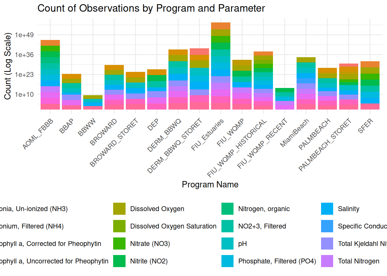
Plot providers row count grouped by analyte

library(ggplot2)

ggplot(df, aes(x = ProgramName, fill = ParameterName)) +
  geom_bar() +
  scale_y_log10() +
  labs(
    title = "Count of Observations by Program and Parameter",
    x = "Program Name",
    y = "Count (Log Scale)",
    fill = "Parameter"
  ) +
  theme_minimal() +
  theme(
    legend.position = "bottom",
    axis.text.x = element_text(angle = 45, hjust = 1)
  )

show n samples from bottom & surface

library(ggplot2)

ggplot(df, aes(x = RelativeDepth)) +
  geom_bar(fill = "steelblue") +
  labs(
    title = "Number of Samples by Relative Depth",
    x = "Relative Depth",
    y = "Number of Samples"
  ) +
  theme_minimal()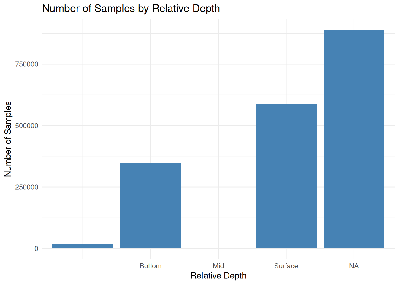

Code

source(here("R/mutateWINToSEACAR.R"))
df <- df_all %>% mutateWINToSEACAR(.keep = "unused")
SEACAR_COLUMNS <- c(
 "ExportVersion","RowID","ProgramID","ProgramName","Habitat",
 "IndicatorID","IndicatorName","ParameterID","ParameterName",
 "ParameterUnits","ProgramLocationID","AreaID","ManagedAreaName",
 "Region","ActivityType","SampleDate","ResultValue","Year","Month",
 "ActivityDepth_m","RelativeDepth","TotalDepth_m","MDL","PQL",
 "DetectionUnit","ValueQualifier","ValueQualifierSource",
 "SampleFraction","ResultComments","OriginalLatitude",
 "OriginalLongitude","SEACAR_QAQCFlagCode",
 "SEACAR_QAQC_Description","Include","SEACAR_EventID","MADup"
)

# figure out which are actually present
present_cols <- intersect(SEACAR_COLUMNS, names(df))
missing_cols <- setdiff(SEACAR_COLUMNS, names(df))

if (length(missing_cols) > 0) {
 warning("\nThese SEACAR_COLUMNS were not found in df:\n  ",
         paste(missing_cols, collapse = ", "))
}

# Any additional columns in df that are not mapped to SEACAR
extra_columns <- setdiff(names(df), SEACAR_COLUMNS)
cat("\nColumns from source data that are not (directly) mapped to SEACAR columns:\n")


Columns from source data that are not (directly) mapped to SEACAR columns:

Code

print(extra_columns)

character(0)