SEACAR Depth Comparisons

Comparison of depth values across SEACAR and older dataset.

Click on any element for more details.

library(here)
library(dplyr)
source(here("SEACARProgramCompare/mapProgramNameToShortName.R"))


# === new dataset
df_SEACAR <- readr::read_delim(
  here("data/Discrete WQ - 10006.txt"),
  delim = "|"
) %>%
  # Convert ActivityDepth_m to numeric for plotting
  mutate(ActivityDepth_m = as.numeric(ActivityDepth_m)) %>%
  # align programName between datasets
  mutate(ProgramName = mapProgramNameToShortName(ProgramName))



# === previous year's dataset
df_OLD <- readr::read_delim(here::here("data/allDataSEACAR.csv"), delim=",") %>%
  # align programName between datasets
  mutate(ProgramName = mapProgramNameToShortName(ProgramName))



# === keep only columns of interest to avoid coltype errors
cols_of_interest <- c(
  "ProgramName", 
  "ActivityDepth_m", 
  "ParameterName",
  "ResultValue", 
  "SampleDate"
)
df_SEACAR <- df_SEACAR %>% select(all_of(cols_of_interest))
df_OLD <- df_OLD %>% select(all_of(cols_of_interest))


# === Combine dataframes with a source column
df_combined <- bind_rows(
  df_SEACAR %>% mutate(source = "SEACAR_STD"),
  df_OLD %>% mutate(source = "OLD_STD")
)

library(ggplot2)
# Create split violin plot
ggplot(df_combined, aes(x = source, y = ActivityDepth_m, fill = source)) +
  geom_violin(alpha = 0.6) +
  geom_boxplot(width = 0.2, alpha = 0.8, outlier.shape = NA) +
  scale_y_log10() +
  labs(
    title = "ActivityDepth_m Distribution Comparison (Log Scale)",
    x = "Dataset",
    y = "ActivityDepth_m (log10)"
  ) +
  theme_minimal() +
  theme(legend.position = "none")

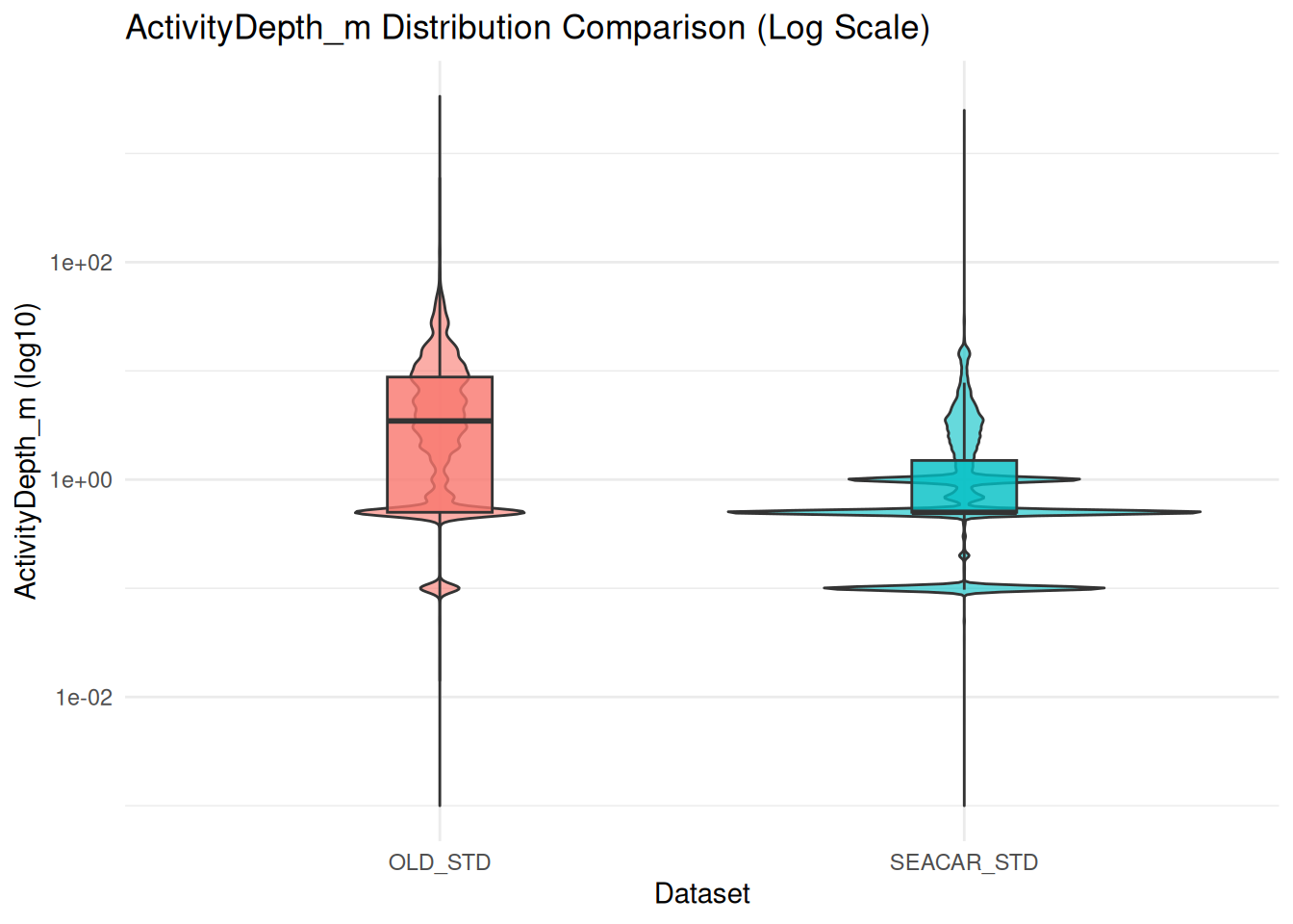
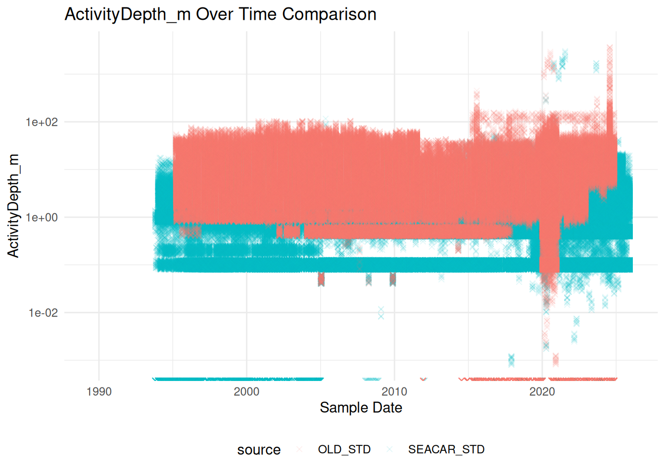
library(ggplot2)

# Create point plot with depth over time
df_combined %>%
# points with x (shape 4), jittered to improve visablity for many overlapping points.
  mutate(depth_jittered = ActivityDepth_m * 10^runif(n(), -0.1, 0.1)) %>%
  ggplot(aes(x = SampleDate, y = depth_jittered, color = source)) +
    geom_point(shape = 4, alpha = 0.1) +
    scale_y_log10() +
    labs(
      title = "ActivityDepth_m Over Time Comparison",
      x = "Sample Date",
      y = "ActivityDepth_m"
    ) +
    theme_minimal() +
    theme(legend.position = "bottom")

---

Random Sample Comparisons

The following is visualization of a random sample of program+parameter combinations.

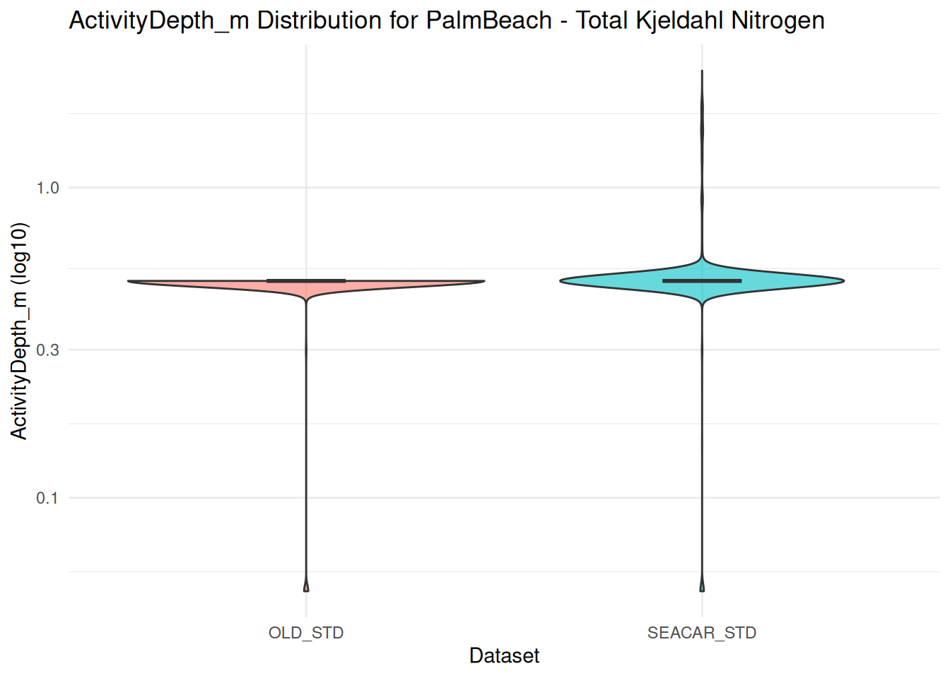
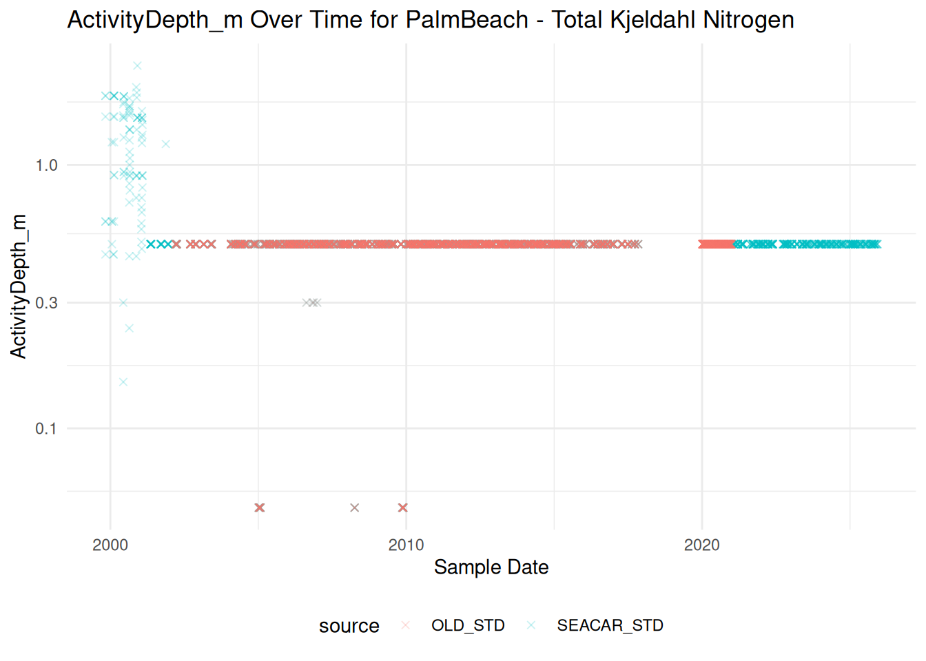
# === 3 parameters from one program
random_program <- sample(unique(df_combined$ProgramName), 1)
program_parameters <- unique(df_combined$ParameterName[df_combined$ProgramName == random_program])
random_parameters <- sample(program_parameters, min(3, length(program_parameters)))

cat("=== Program:", random_program, "===\n")

=== Program: PalmBeach ===

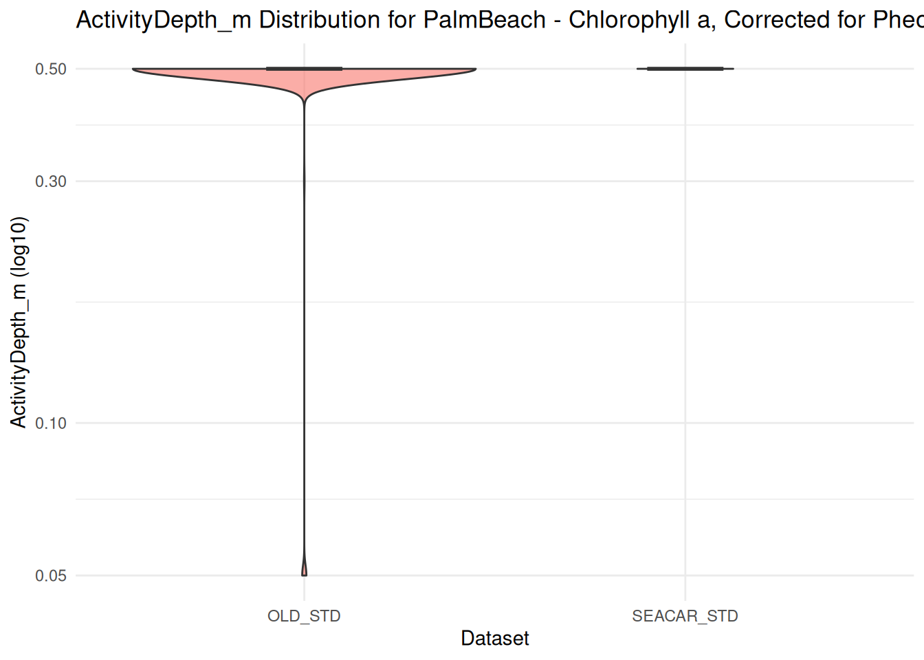
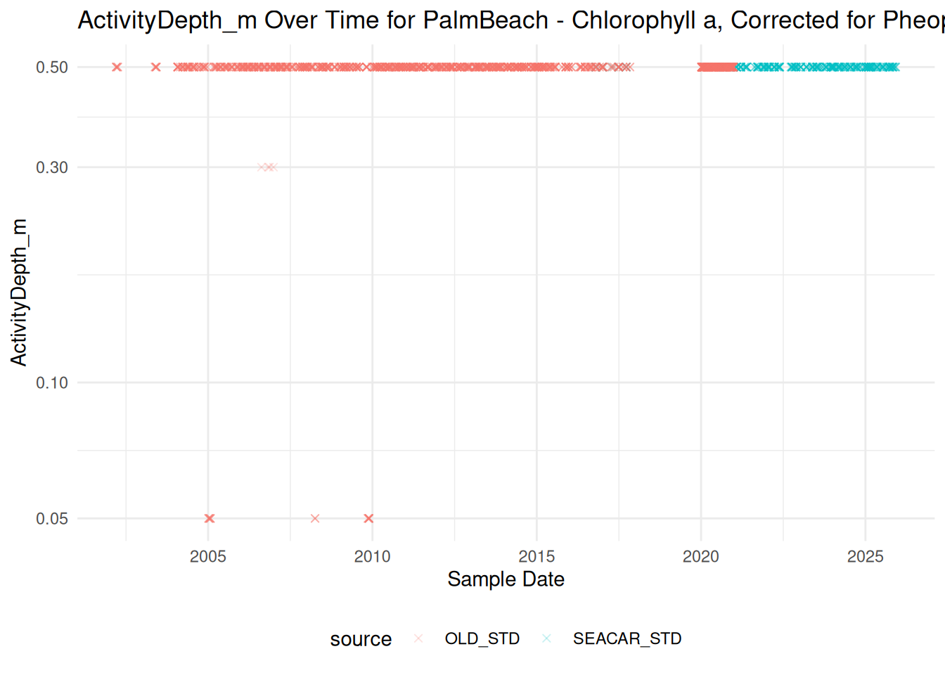
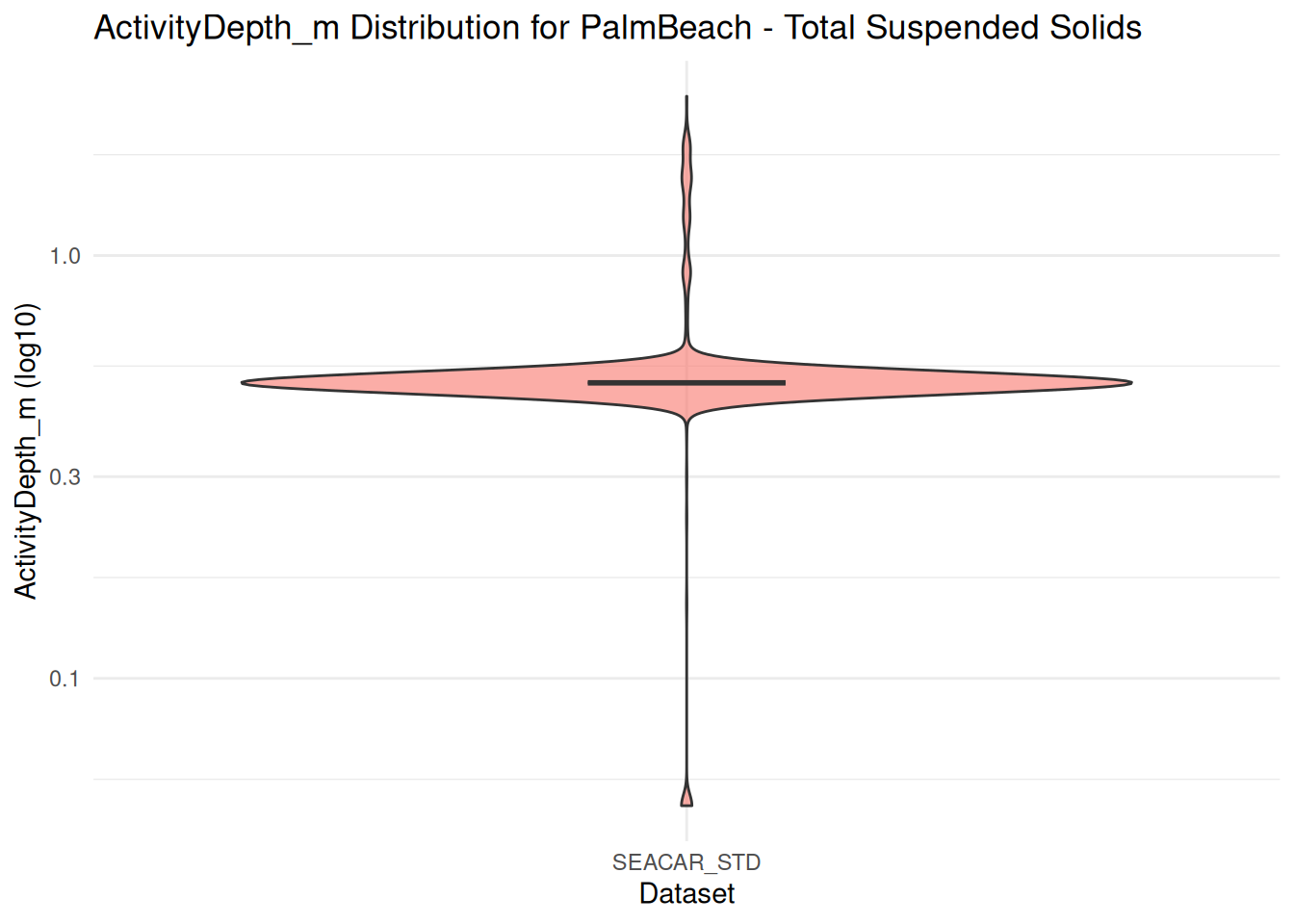
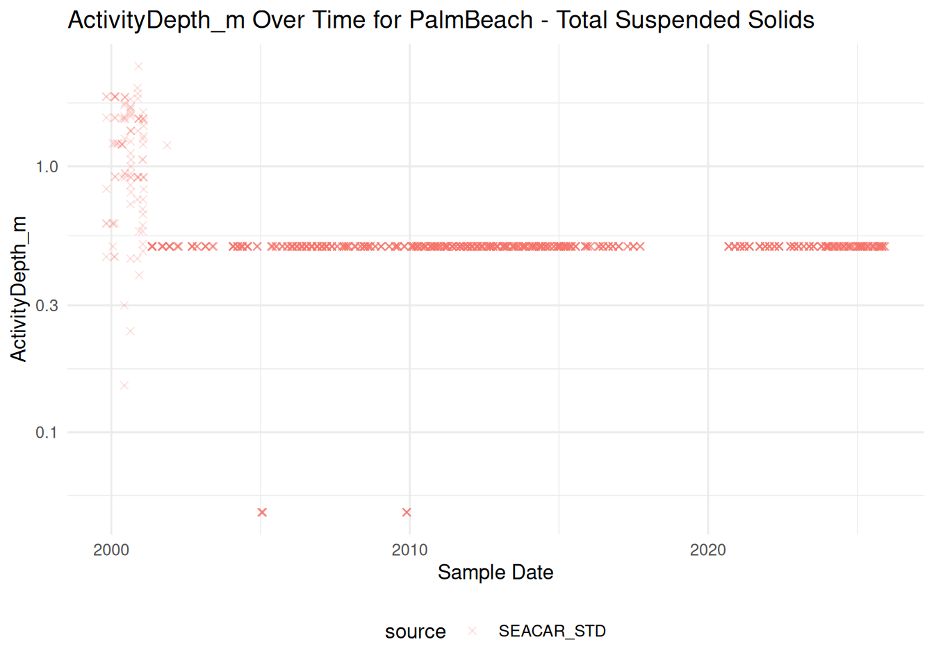
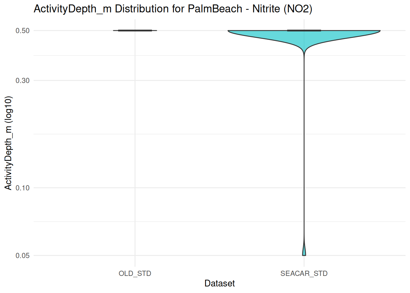
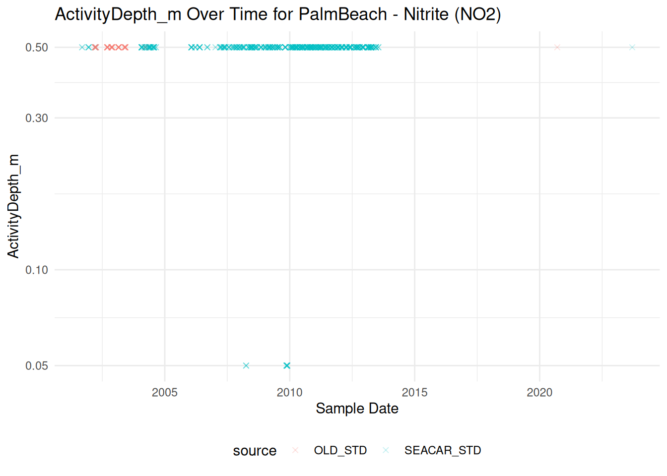
for (i in 1:length(random_parameters)) {
  random_parameter <- random_parameters[i]
  
  df_subset <- df_combined %>%
    filter(ProgramName == random_program, ParameterName == random_parameter)
  
  cat("Parameter:", random_parameter, "\n")
  
  # === violin plot
  p1 <- ggplot(df_subset, aes(x = source, y = ActivityDepth_m, fill = source)) +
    geom_violin(alpha = 0.6) +
    geom_boxplot(width = 0.2, alpha = 0.8, outlier.shape = NA) +
    scale_y_log10() +
    labs(
      title = paste("ActivityDepth_m Distribution for", random_program, "-", random_parameter),
      x = "Dataset",
      y = "ActivityDepth_m (log10)"
    ) +
    theme_minimal() +
    theme(legend.position = "none")
  
  print(p1)
  
  # === time series plot
  p2 <- ggplot(df_subset, aes(x = SampleDate, y = ActivityDepth_m, color = source)) +
    geom_point(shape = 4, alpha = 0.2) +
    scale_y_log10() +
    labs(
      title = paste("ActivityDepth_m Over Time for", random_program, "-", random_parameter),
      x = "Sample Date",
      y = "ActivityDepth_m"
    ) +
    theme_minimal() +
    theme(legend.position = "bottom")
  
  print(p2)
}

Parameter: Total Kjeldahl Nitrogen 

Parameter: Chlorophyll a, Corrected for Pheophytin 

Parameter: Total Suspended Solids 

# === 3 programs for one parameter
random_parameter <- sample(unique(df_combined$ParameterName), 1)
parameter_programs <- unique(df_combined$ProgramName[df_combined$ParameterName == random_parameter])
random_programs <- sample(parameter_programs, min(3, length(parameter_programs)))

cat("\n=== Parameter:", random_parameter, "===\n")

=== Parameter: Nitrite (NO2) ===

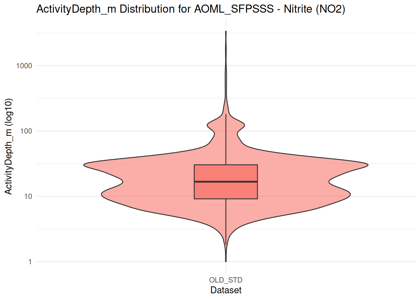
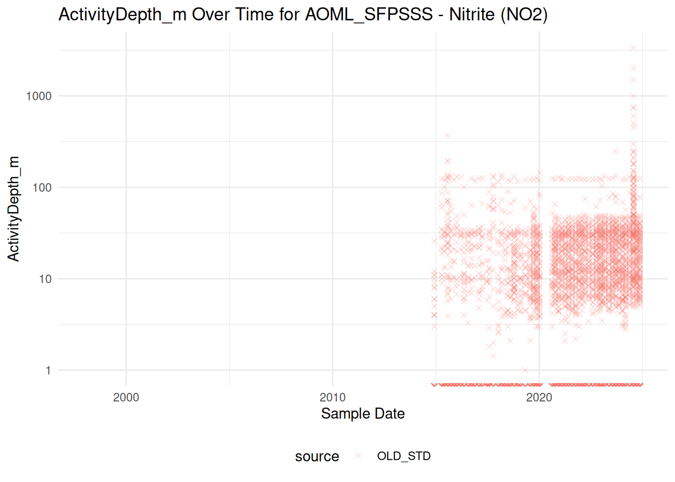
for (i in 1:length(random_programs)) {
  random_program <- random_programs[i]
  
  df_subset <- df_combined %>%
    filter(ProgramName == random_program, ParameterName == random_parameter)
  
  cat("Program:", random_program, "\n")
  
  # === violin plot
  p1 <- ggplot(df_subset, aes(x = source, y = ActivityDepth_m, fill = source)) +
    geom_violin(alpha = 0.6) +
    geom_boxplot(width = 0.2, alpha = 0.8, outlier.shape = NA) +
    scale_y_log10() +
    labs(
      title = paste("ActivityDepth_m Distribution for", random_program, "-", random_parameter),
      x = "Dataset",
      y = "ActivityDepth_m (log10)"
    ) +
    theme_minimal() +
    theme(legend.position = "none")
  
  print(p1)
  
  # === time series plot
  p2 <- ggplot(df_subset, aes(x = SampleDate, y = ActivityDepth_m, color = source)) +
    geom_point(shape = 4, alpha = 0.2) +
    scale_y_log10() +
    labs(
      title = paste("ActivityDepth_m Over Time for", random_program, "-", random_parameter),
      x = "Sample Date",
      y = "ActivityDepth_m"
    ) +
    theme_minimal() +
    theme(legend.position = "bottom")
  
  print(p2)
}

Program: PalmBeach 

Program: AOML_SFPSSS 

Program: SE_FL_WQAS