SEACARParameterCompare

Reports for each value in the batch.

Click on any element for more details.

library(here)
df_SEACAR <- readr::read_delim(
  here("data/Discrete WQ - 10006.txt"),
  delim = "|"
)
df_OLD <- readr::read_delim(here::here("data/allDataSEACAR.csv"), delim=",")

library(dplyr)

u1 <- unique(df_SEACAR$ParameterName)
u2 <- unique(df_OLD$ParameterName)

comparison <- tibble(value = union(u1, u2)) %>%
  mutate(
    in_SEACAR = value %in% u1,
    in_OLD    = value %in% u2
  )

print(comparison, n=100)

# A tibble: 26 × 3
   value                                     in_SEACAR in_OLD
   <chr>                                     <lgl>     <lgl> 
 1 Salinity                                  TRUE      TRUE  
 2 Water Temperature                         TRUE      TRUE  
 3 pH                                        TRUE      TRUE  
 4 Total Suspended Solids                    TRUE      TRUE  
 5 Chlorophyll a, Corrected for Pheophytin   TRUE      TRUE  
 6 Light Extinction Coefficient              TRUE      FALSE 
 7 Colored Dissolved Organic Matter          TRUE      FALSE 
 8 NO2+3, Filtered                           TRUE      TRUE  
 9 Ammonium (NH4)                            TRUE      FALSE 
10 Phosphate, Filtered (PO4)                 TRUE      TRUE  
11 Dissolved Oxygen                          TRUE      TRUE  
12 Dissolved Oxygen Saturation               TRUE      TRUE  
13 Turbidity                                 TRUE      TRUE  
14 Chlorophyll a, Uncorrected for Pheophytin TRUE      TRUE  
15 Total Nitrogen                            TRUE      TRUE  
16 Total Phosphorus                          TRUE      TRUE  
17 Nitrate (NO3)                             TRUE      TRUE  
18 Nitrite (NO2)                             TRUE      TRUE  
19 Nitrogen, organic                         TRUE      TRUE  
20 Total Ammonia (N)                         TRUE      FALSE 
21 Nitrogen, inorganic                       TRUE      FALSE 
22 Specific Conductivity                     TRUE      TRUE  
23 Total Kjeldahl Nitrogen                   TRUE      TRUE  
24 Secchi Depth                              TRUE      FALSE 
25 Ammonium, Filtered (NH4)                  FALSE     TRUE  
26 Ammonia, Un-ionized (NH3)                 FALSE     TRUE  

library(ggplot2)
library(tidyr)

# Count rows by ParameterName for SEACAR dataset
seacar_parameter_counts <- df_SEACAR %>%
  group_by(ParameterName) %>%
  count(name = "SEACAR_Count") %>%
  arrange(desc(SEACAR_Count))

# Count rows by ParameterName for OLD dataset
old_parameter_counts <- df_OLD %>%
  group_by(ParameterName) %>%
  count(name = "OLD_Count") %>%
  arrange(desc(OLD_Count))

# Create combined dataframe for plotting
combined_parameter_counts <- full_join(
  seacar_parameter_counts,
  old_parameter_counts,
  by = "ParameterName"
) %>%
  mutate(
    SEACAR_Count = replace_na(SEACAR_Count, 0),
    OLD_Count = replace_na(OLD_Count, 0)
  ) %>%
  # Reshape to long format for dodged bars
  pivot_longer(
    cols = c(SEACAR_Count, OLD_Count),
    names_to = "source",
    values_to = "count"
  ) %>%
  mutate(source = ifelse(source == "SEACAR_Count", "SEACAR_STD", "OLD"))

# === Split the plot into two because there are many parameters
TEXT_ANGLE = 90
# Split parameters alphabetically
parameters <- unique(combined_parameter_counts$ParameterName)
mid_point <- ceiling(length(parameters) / 2)
first_half <- sort(parameters)[1:mid_point]
second_half <- sort(parameters)[(mid_point + 1):length(parameters)]

# Create first plot (A-M)
plot1_data <- combined_parameter_counts %>%
  filter(ParameterName %in% first_half) %>%
  mutate(ParameterName = factor(ParameterName, levels = sort(first_half)))

plot1 <- ggplot(plot1_data, aes(x = ParameterName, y = count, fill = source)) +
  geom_bar(stat = "identity", position = "dodge") +
  labs(
    title = "Row Count by ParameterName (A-M)",
    x = "ParameterName",
    y = "Number of Rows",
    fill = "Dataset"
  ) +
  theme_minimal() + 
  theme(axis.text.x = element_text(angle = TEXT_ANGLE, hjust = 1))

# Create second plot (N-Z)
plot2_data <- combined_parameter_counts %>%
  filter(ParameterName %in% second_half) %>%
  mutate(ParameterName = factor(ParameterName, levels = sort(second_half)))

plot2 <- ggplot(plot2_data, aes(x = ParameterName, y = count, fill = source)) +
  geom_bar(stat = "identity", position = "dodge") +
  labs(
    title = "Row Count by ParameterName (N-Z)",
    x = "ParameterName",
    y = "Number of Rows",
    fill = "Dataset"
  ) +
  theme_minimal() + 
  theme(axis.text.x = element_text(angle = TEXT_ANGLE, hjust = 1))

# Display both plots
print(plot1)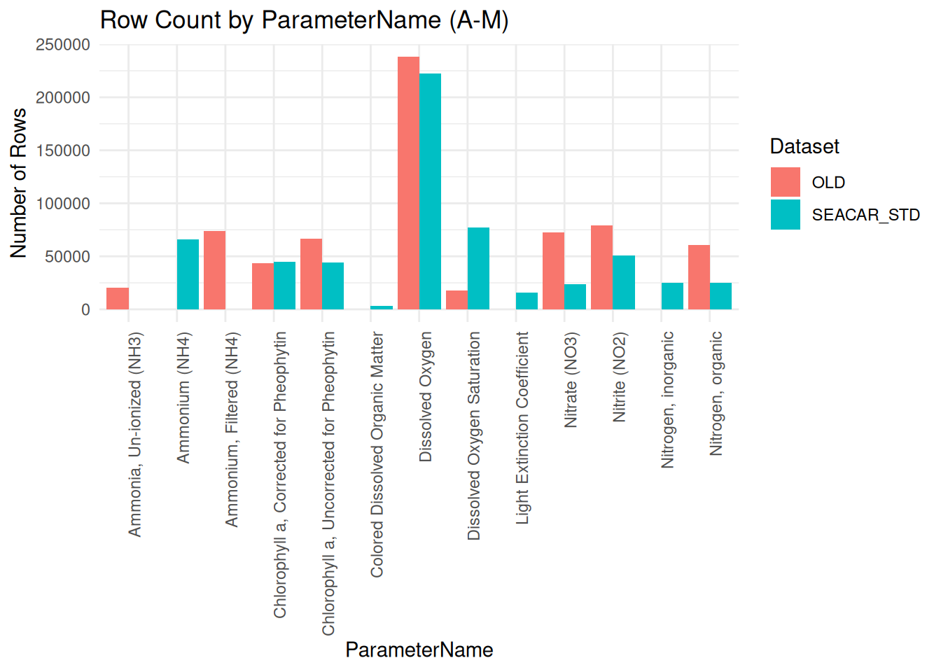

print(plot2)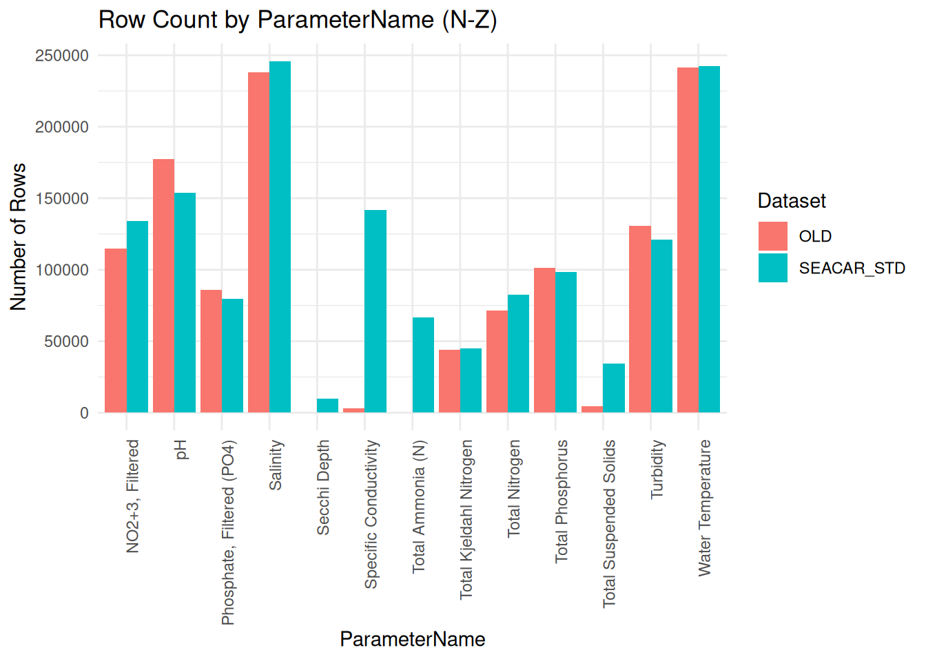

c1 <- colnames(df_SEACAR)
c2 <- colnames(df_OLD)

comparison <- data.frame(
  column = union(c1, c2),
  in_SEACAR = union(c1, c2) %in% c1,
  in_OLD    = union(c1, c2) %in% c2
)

print(comparison)

                    column in_SEACAR in_OLD
1                    RowID      TRUE   TRUE
2                ProgramID      TRUE   TRUE
3              ProgramName      TRUE   TRUE
4                  Habitat      TRUE   TRUE
5              IndicatorID      TRUE   TRUE
6            IndicatorName      TRUE   TRUE
7              ParameterID      TRUE   TRUE
8            ParameterName      TRUE   TRUE
9           ParameterUnits      TRUE   TRUE
10             ResultValue      TRUE   TRUE
11              SampleDate      TRUE   TRUE
12                    Year      TRUE   TRUE
13                   Month      TRUE   TRUE
14     SEACAR_QAQCFlagCode      TRUE   TRUE
15 SEACAR_QAQC_Description      TRUE   TRUE
16                 Include      TRUE   TRUE
17              LocationID      TRUE  FALSE
18       ProgramLocationID      TRUE   TRUE
19     ProgramLocationName      TRUE  FALSE
20        OriginalLatitude      TRUE   TRUE
21       OriginalLongitude      TRUE   TRUE
22                  AreaID      TRUE   TRUE
23         ManagedAreaName      TRUE   TRUE
24             AreaID_Buff      TRUE  FALSE
25    ManagedAreaName_Buff      TRUE  FALSE
26         EstuarineMarine      TRUE  FALSE
27                   OIMMP      TRUE  FALSE
28                  CHIMMP      TRUE  FALSE
29             CoralRegion      TRUE  FALSE
30            ActivityType      TRUE   TRUE
31         ActivityDepth_m      TRUE   TRUE
32           RelativeDepth      TRUE   TRUE
33            TotalDepth_m      TRUE   TRUE
34                     MDL      TRUE   TRUE
35                     PQL      TRUE   TRUE
36           DetectionUnit      TRUE   TRUE
37          ValueQualifier      TRUE   TRUE
38    ValueQualifierSource      TRUE   TRUE
39          SampleFraction      TRUE  FALSE
40          ResultComments      TRUE   TRUE
41          SEACAR_EventID      TRUE   TRUE
42           ExportVersion      TRUE   TRUE
43                    ...1     FALSE   TRUE
44                   MADup     FALSE   TRUE
45                  Region     FALSE   TRUE

library(ggplot2)
library(tidyr)
library(lubridate)

# Count rows per date for each dataset, bin by year
seacar_counts <- df_SEACAR %>%
  group_by(SampleDate = floor_date(SampleDate, "year")) %>%
  count(name = "SEACAR_Count") %>%
  ungroup()

old_counts <- df_OLD %>%
  group_by(SampleDate = floor_date(SampleDate, "year")) %>%
  count(name = "OLD_Count") %>%
  ungroup()

# Combine and plot
combined_counts <- full_join(seacar_counts, old_counts, by = "SampleDate") %>%
  arrange(SampleDate) %>%
  mutate(
    SEACAR_Count = replace_na(SEACAR_Count, 0),
    OLD_Count = replace_na(OLD_Count, 0)
  )

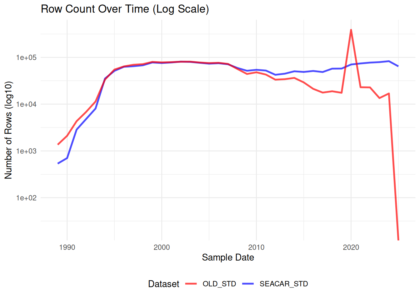
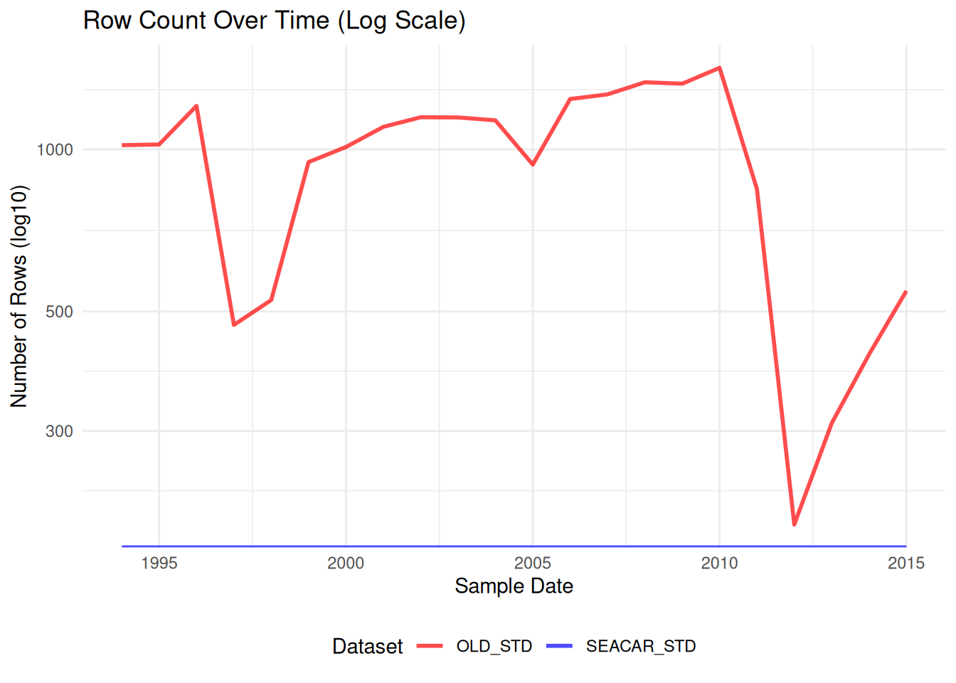
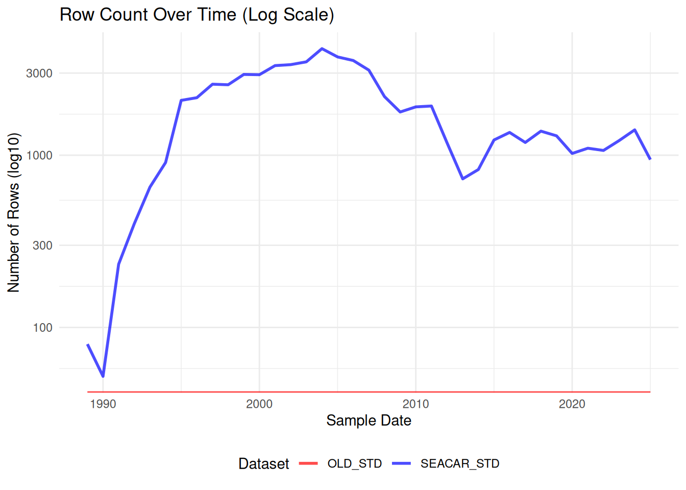
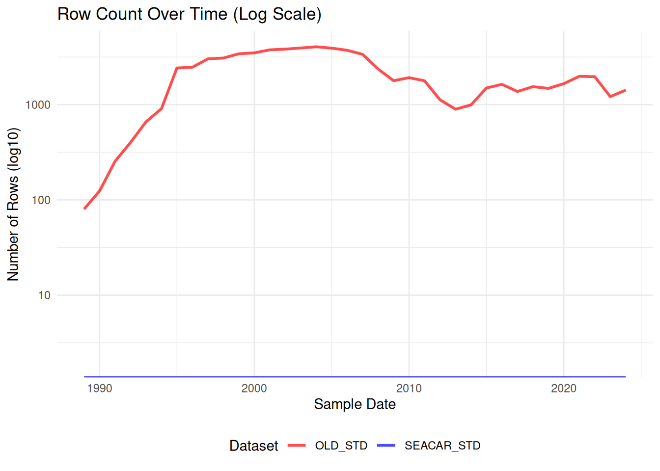
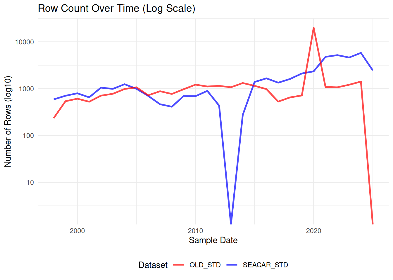
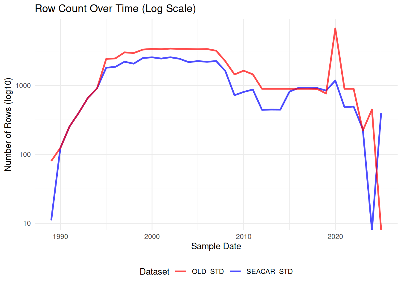
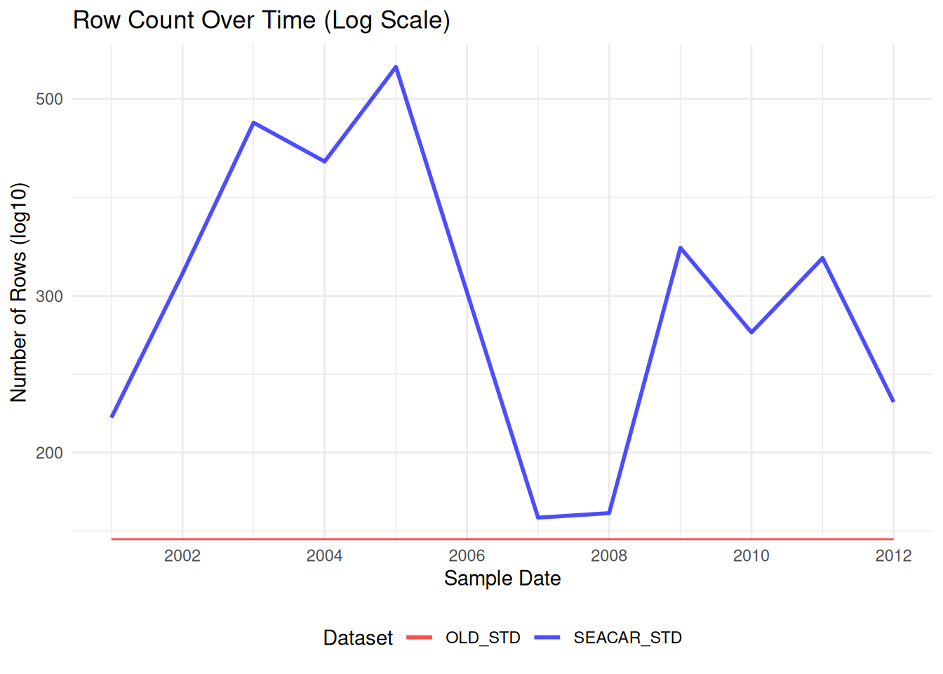
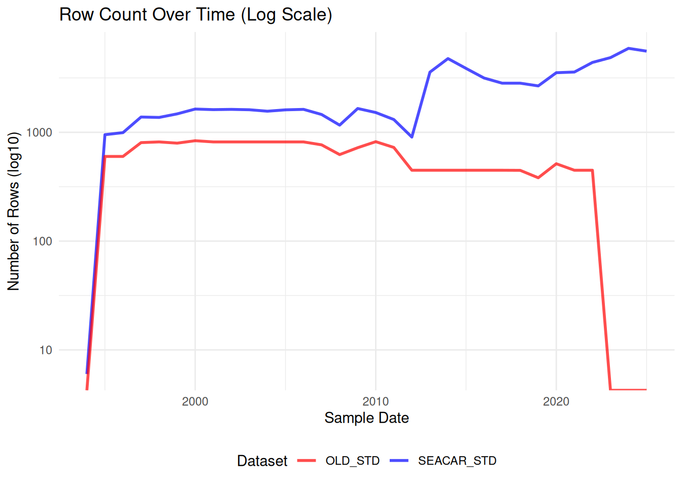
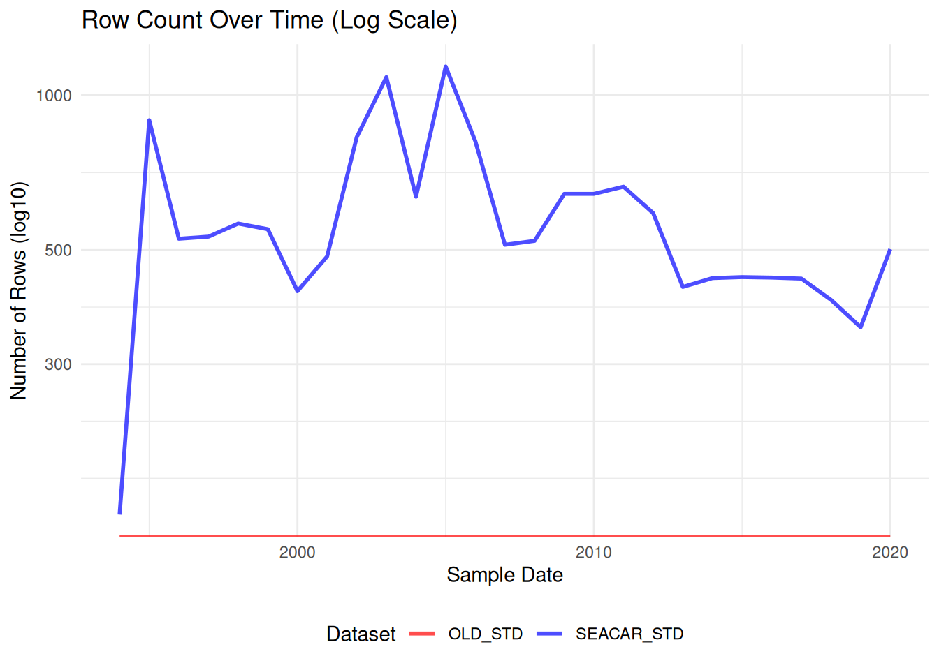
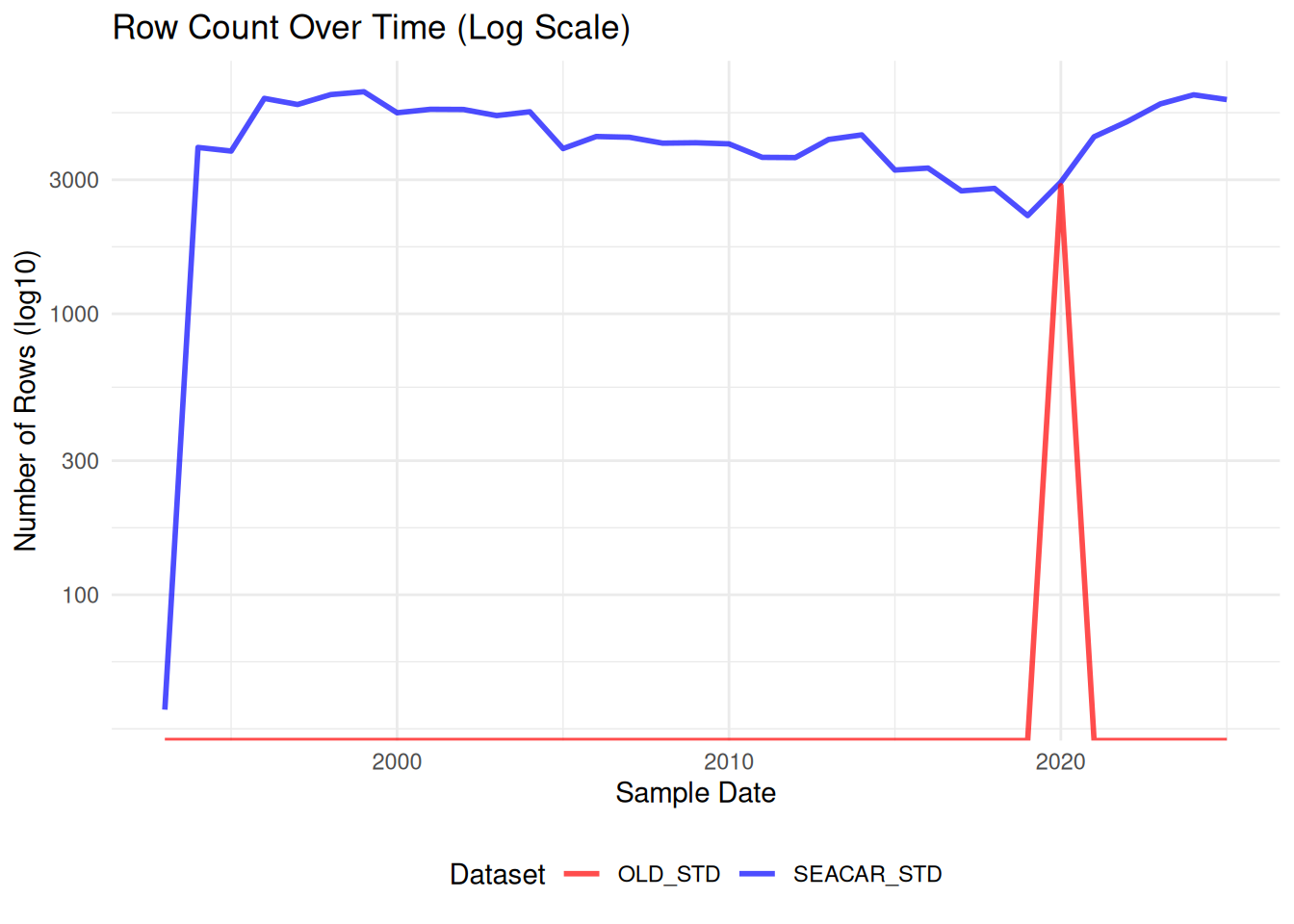
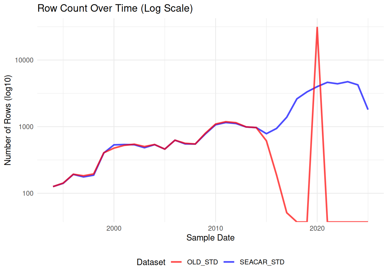
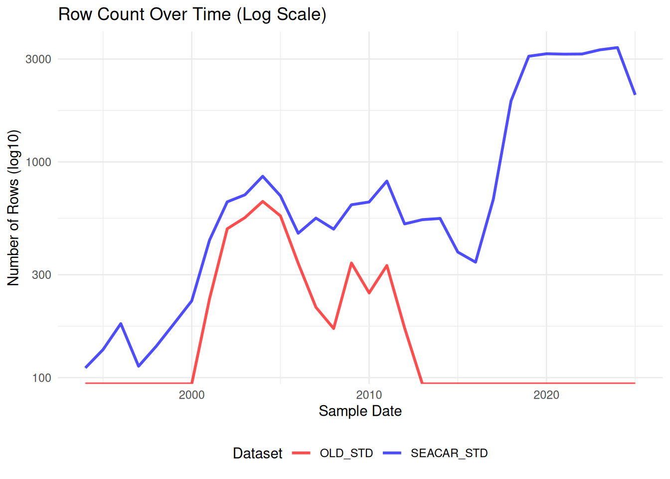
ggplot(combined_counts, aes(x = SampleDate)) +
  geom_line(aes(y = SEACAR_Count, color = "SEACAR_STD", linetype = "SEACAR_STD"), size = 1, alpha = 0.7) +
  geom_line(aes(y = OLD_Count, color = "OLD_STD", linetype = "OLD_STD"), size = 1, alpha = 0.7) +
  scale_y_log10() +
  scale_linetype_manual(values = c("SEACAR_STD" = "solid", "OLD_STD" = "solid")) +
  scale_color_manual(values = c("SEACAR_STD" = "blue", "OLD_STD" = "red")) +
  labs(
    title = "Row Count Over Time (Log Scale)",
    x = "Sample Date",
    y = "Number of Rows (log10)",
    color = "Dataset",
    linetype = "Dataset"
  ) +
  theme_minimal() +
  theme(legend.position = "bottom")