FKNMS Report

source(here::here(glue::glue("{params$batch_name}/getData.R")))

# returns two dataframes in a named list
dfs <- getData(params$batch_value)

# keep only columns of interest
cols_of_interest <- c(
  "ProgramName", "ProgramLocationID", "OriginalLatitude", "OriginalLongitude", 
  "ActivityDepth_m", "ParameterUnits", "ParameterName", "ResultValue", "SampleDate"
)
dfs$SEACAR_STD <- dfs$SEACAR_STD %>% select(all_of(cols_of_interest))
dfs$OLD <- dfs$OLD %>% select(all_of(cols_of_interest))

Row Counts

cat(" SEACAR_STD rows:", nrow(dfs$SEACAR_STD), "\n")

 SEACAR_STD rows: 472109 

cat("OLD dataset rows:", nrow(dfs$OLD), "\n")

OLD dataset rows: 550859 

library(ggplot2)
library(tidyr)
library(lubridate)

# Count rows per date for each dataset, bin by year
seacar_counts <- dfs$SEACAR_STD %>%
  group_by(SampleDate = floor_date(SampleDate, "year")) %>%
  count(name = "SEACAR_Count") %>%
  ungroup()

old_counts <- dfs$OLD %>%
  group_by(SampleDate = floor_date(SampleDate, "year")) %>%
  count(name = "OLD_Count") %>%
  ungroup()

# Combine and plot
combined_counts <- full_join(seacar_counts, old_counts, by = "SampleDate") %>%
  arrange(SampleDate) %>%
  mutate(
    SEACAR_Count = replace_na(SEACAR_Count, 0),
    OLD_Count = replace_na(OLD_Count, 0)
  )

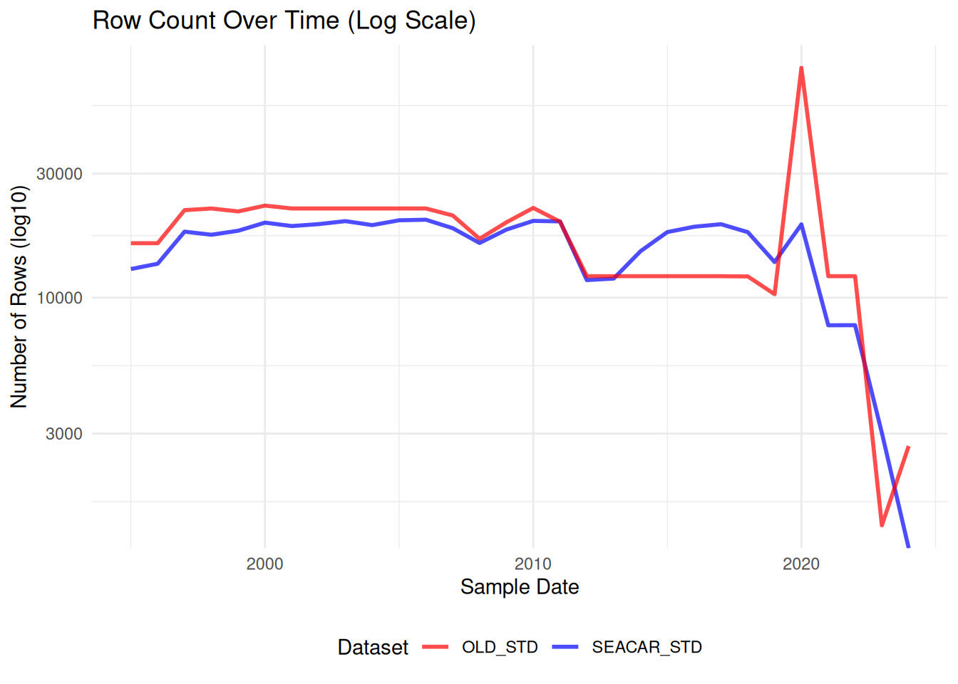
ggplot(combined_counts, aes(x = SampleDate)) +
  geom_line(aes(y = SEACAR_Count, color = "SEACAR_STD", linetype = "SEACAR_STD"), size = 1, alpha = 0.7) +
  geom_line(aes(y = OLD_Count, color = "OLD_STD", linetype = "OLD_STD"), size = 1, alpha = 0.7) +
  scale_y_log10() +
  scale_linetype_manual(values = c("SEACAR_STD" = "solid", "OLD_STD" = "solid")) +
  scale_color_manual(values = c("SEACAR_STD" = "blue", "OLD_STD" = "red")) +
  labs(
    title = "Row Count Over Time (Log Scale)",
    x = "Sample Date",
    y = "Number of Rows (log10)",
    color = "Dataset",
    linetype = "Dataset"
  ) +
  theme_minimal() +
  theme(legend.position = "bottom")

Result Value Comparison

Distribution of ResultValues

library(ggplot2)

if (nrow(dfs$SEACAR_STD) == 0 || nrow(dfs$OLD) == 0) {
  cat("One or both dataframes are empty.\n")
} else {
  # Combine dataframes with a source column
  df_combined <- bind_rows(
    dfs$SEACAR_STD %>% mutate(source = "SEACAR_STD"),
    dfs$OLD %>% mutate(source = "OLD_STD")
  )

  # Create split violin plot
  ggplot(df_combined, aes(x = source, y = ResultValue, fill = source)) +
    geom_violin(alpha = 0.6) +
    geom_boxplot(width = 0.2, alpha = 0.8, outlier.shape = NA) +
    scale_y_log10() +
    labs(
      title = "Value Distribution Comparison (Log Scale)",
      x = "Dataset",
      y = "Result Value (log10)"
    ) +
    theme_minimal() +
    theme(legend.position = "none")
}

ResultValues over time

This plots the value recorded across all parameters for both datasets. Differences throughout time could be from changes in protocols. For example: if a parameter is recorded for only part of the time series.

library(ggplot2)

if (nrow(dfs$SEACAR_STD) == 0 || nrow(dfs$OLD) == 0) {
  cat("One or both dataframes are empty.\n")
} else {
  # Combine dataframes with a source column
  df_combined <- bind_rows(
    dfs$SEACAR_STD %>% mutate(source = "SEACAR_STD"),
    dfs$OLD %>% mutate(source = "OLD_STD")
  ) %>% 
    filter(ParameterName == "Salinity")

  ggplot(df_combined, aes(x = SampleDate, y = ResultValue, color = source)) +
    geom_point(alpha = 0.3, shape=4) +
    scale_y_log10() +
    labs(
      title = "salinity Over Time",
      x = "Sample Date",
      y = "salinity"
    ) +
    theme_minimal() +
    theme(legend.position = "bottom")
}

Depth Distributions

library(ggplot2)

if (nrow(dfs$SEACAR_STD) == 0 || nrow(dfs$OLD) == 0) {
  cat("One or both dataframes are empty.\n")
} else {
  # Combine dataframes with a source column
  df_combined <- bind_rows(
    dfs$SEACAR_STD %>% mutate(source = "SEACAR_STD"),
    dfs$OLD %>% mutate(source = "OLD_STD")
  )

  # Create split violin plot
  ggplot(df_combined, aes(x = source, y = ActivityDepth_m, fill = source)) +
    geom_violin(alpha = 0.6) +
    geom_boxplot(width = 0.2, alpha = 0.8, outlier.shape = NA) +
    scale_y_log10() +
    labs(
      title = "ActivityDepth_m Distribution Comparison (Log Scale)",
      x = "Dataset",
      y = "ActivityDepth_m (log10)"
    ) +
    theme_minimal() +
    theme(legend.position = "none")
}

ProgramLocationID Alignment

library(dplyr)

# Find ProgramLocationIDs that exist only in only one of the datasets
seacar_only <- setdiff(dfs$SEACAR_STD$ProgramLocationID, dfs$OLD$ProgramLocationID)
old_only <- setdiff(dfs$OLD$ProgramLocationID, dfs$SEACAR_STD$ProgramLocationID)


# plot counts of unique ProgramLocationIDs in OLD, SEACAR_STD, and both
library(ggplot2)
both        <- intersect(dfs$SEACAR_STD$ProgramLocationID, dfs$OLD$ProgramLocationID)

venn_df <- data.frame(
  group = c("SEACAR only", "Both", "OLD only"),
  count = c(length(seacar_only), length(both), length(old_only))
)

ggplot(venn_df, aes(x = group, y = count, fill = group)) +
  geom_col(width = 0.6) +
  geom_text(aes(label = count), vjust = -0.5, size = 4) +
  scale_fill_manual(values = c(
    "SEACAR only" = "#378ADD",
    "Both"        = "#999E75",
    "OLD only"    = "#FFCAA5"
  )) +
  scale_x_discrete(limits = c("SEACAR only", "Both", "OLD only")) +
  labs(
    title = "ProgramLocationID overlap between SEACAR and OLD datasets",
    x = NULL,
    y = "Number of unique ProgramLocationIDs"
  ) +
  theme_minimal() +
  theme(legend.position = "none")

# cat("Number of ProgramLocationIDs in SEACAR_STD but not in OLD_STD:", length(seacar_only), "/", length(unique(dfs$SEACAR_STD$ProgramLocationID)), "\n")
cat("First few ProgramLocationIDs in SEACAR_STD but not in OLD_STD:", head(seacar_only), "\n")

First few ProgramLocationIDs in SEACAR_STD but not in OLD_STD:  

# cat("Number of ProgramLocationIDs in OLD_STD but not in SEACAR_STD:", length(old_only), "/", length(unique(dfs$OLD$ProgramLocationID)), "\n")
cat("First few ProgramLocationIDs in OLD_STD but not in SEACAR_STD:", head(old_only), "\n")

First few ProgramLocationIDs in OLD_STD but not in SEACAR_STD: 281i