Tidy Wide Format

The default data file is in “long” format, with “analyte name” as a column. This document transforms the data to “wide” “tidy” format, with “analyte name” on the columns. This is done by pivoting on the analyte name column.

if (!requireNamespace("librarian", quietly = TRUE)) {
  install.packages("librarian")
}
librarian::shelf(
  dplyr,
  tidyr,
  here,
  readr,
  ggplot2,
  skimr
)

source(here("SEACARProgramCompare/mapProgramNameToShortName.R"))

df_long <- readr::read_delim(
  here("data/Discrete WQ - 10006.txt"),
  delim = "|"
) %>%
  mutate(ProgramName = mapProgramNameToShortName(ProgramName))


# Show dimensions of long format data
cat("Long format dimensions:\n")

Long format dimensions:

cat("  Rows:", nrow(df_long), "\n")

  Rows: 2085902 

cat("  Columns:", ncol(df_long), "\n")

  Columns: 42 

Transform to Wide Format

Pre-Pivot Collision Check

Before pivoting we assess how many collisions will occur.

df_long %>%
  group_by(ProgramName, ProgramLocationID, SampleDate, ActivityDepth_m, ParameterName) %>%
  summarise(n = n(), .groups = "drop") %>%
  filter(n > 1)

# A tibble: 262,886 × 6
   ProgramName ProgramLocationID SampleDate          ActivityDepth_m
   <chr>       <chr>             <dttm>              <chr>          
 1 AOML_SFPSSS 1                 1998-01-20 00:00:00 NULL           
 2 AOML_SFPSSS 1                 1998-01-20 00:00:00 NULL           
 3 AOML_SFPSSS 1                 1998-03-10 00:00:00 NULL           
 4 AOML_SFPSSS 1                 1998-03-10 00:00:00 NULL           
 5 AOML_SFPSSS 1                 1998-06-30 00:00:00 NULL           
 6 AOML_SFPSSS 1                 1998-06-30 00:00:00 NULL           
 7 AOML_SFPSSS 1                 2014-12-01 13:23:00 NULL           
 8 AOML_SFPSSS 1                 2015-06-01 12:09:00 NULL           
 9 AOML_SFPSSS 1                 2015-07-27 12:20:00 NULL           
10 AOML_SFPSSS 1                 2015-09-21 13:01:00 NULL           
# ℹ 262,876 more rows
# ℹ 2 more variables: ParameterName <chr>, n <int>

These rows will collide with n other rows (see column on far right). An example cause of this is samples that were taken at the same time on the same day. Collisions in this pivot are averaged with a mean.

Pivot

The transformation uses tidyr::pivot_wider() to convert the dataset from long format (where each row is one measurement of one analyte) to wide format (where each row represents all measurements at a specific location and time).

library(dplyr)
library(tidyr)

# Pivot to wide format using the actual column names from dashboardData.csv
df_wide <- df_long %>%
  pivot_wider(
    id_cols = c(
      ProgramName, 
      ProgramLocationID, 
      SampleDate, 
      ParameterUnits, 
      OriginalLatitude, 
      OriginalLongitude, 
      ActivityDepth_m
    ),
    names_from = ParameterName,
    values_from = ResultValue,
    values_fn = mean  # aggregate duplicates by taking mean
  )

# Show dimensions of wide format data
cat("Wide format dimensions:\n")

Wide format dimensions:

cat("  Rows:", nrow(df_wide), "\n")

  Rows: 1233499 

cat("  Columns:", ncol(df_wide), "\n")

  Columns: 31 

cat("\nNumber of analyte columns created:", ncol(df_wide) - 7, "\n")

Number of analyte columns created: 24 

Preview Wide Format Data

# Display first 100 rows with scrolling
DT::datatable(
  head(df_wide, 100),
  options = list(
    scrollX = TRUE,
    scrollY = "400px",
    pageLength = 10
  ),
  caption = "First 100 rows of wide format data (scroll to see all columns)"
)

library(skimr)

# Skim the numeric columns (analyte measurements)
numeric_cols <- sapply(df_wide, is.numeric)
if (sum(numeric_cols) > 0) {
  cat("Summary of numeric analyte columns:\n\n")
  skim(df_wide[, numeric_cols])
} else {
  cat("No numeric columns found in wide format data.\n")
}

Summary of numeric analyte columns:

Data summary

Name	df_wide[, numeric_cols]
Number of rows	1233499
Number of columns	26
_______________________
Column type frequency:
numeric	26
________________________
Group variables	None

Variable type: numeric

skim_variable	n_missing	complete_rate	mean	sd	p0	p25	p50	p75	p100	hist
OriginalLatitude	0	1.00	25.58	0.48	23.86	25.26	25.64	25.85	28.78	▁▇▃▁▁
OriginalLongitude	0	1.00	-80.52	0.55	-85.02	-80.54	-80.32	-80.18	-79.84	▁▁▁▂▇
Salinity	1029182	0.17	22.77	92.69	-0.01	3.50	29.60	35.39	41361.00	▇▁▁▁▁
Water Temperature	1032325	0.16	26.23	7.31	2.78	23.85	26.47	29.00	2902.00	▇▁▁▁▁
pH	1081701	0.12	7.82	3.99	1.52	7.49	7.89	8.09	820.00	▇▁▁▁▁
Total Suspended Solids	1197940	0.03	8.41	33.67	0.00	1.64	3.47	5.00	4030.00	▇▁▁▁▁
Chlorophyll a, Corrected for Pheophytin	1200293	0.03	1.42	2.89	0.00	0.35	0.59	1.33	64.40	▇▁▁▁▁
Light Extinction Coefficient	1217866	0.01	0.43	0.66	0.00	0.12	0.26	0.49	26.42	▇▁▁▁▁
Colored Dissolved Organic Matter	1230012	0.00	19.54	13.62	0.00	9.94	16.77	26.09	149.02	▇▂▁▁▁
NO2+3, Filtered	1109000	0.10	0.18	1.03	-0.01	0.00	0.01	0.06	81.30	▇▁▁▁▁
Ammonium (NH4)	1178867	0.04	0.36	1.61	0.00	0.00	0.01	0.07	160.80	▇▁▁▁▁
Phosphate, Filtered (PO4)	1172973	0.05	0.03	0.09	0.00	0.00	0.01	0.03	7.67	▇▁▁▁▁
Dissolved Oxygen	1050300	0.15	5.62	13.56	-41.17	4.51	5.92	6.71	5389.00	▇▁▁▁▁
Dissolved Oxygen Saturation	1171844	0.05	74.46	28.97	0.28	56.40	84.92	96.00	585.70	▇▁▁▁▁
Turbidity	1119634	0.09	2.11	5.49	-0.52	0.40	0.90	2.10	495.76	▇▁▁▁▁
Chlorophyll a, Uncorrected for Pheophytin	1188611	0.04	1.60	2.43	0.00	0.26	0.57	1.90	55.12	▇▁▁▁▁
Total Nitrogen	1161876	0.06	0.50	0.74	0.00	0.16	0.30	0.60	52.06	▇▁▁▁▁
Total Phosphorus	1141724	0.07	0.85	77.24	-0.01	0.01	0.01	0.02	11891.04	▇▁▁▁▁
Nitrate (NO3)	1217347	0.01	0.02	0.46	0.00	0.00	0.00	0.00	34.00	▇▁▁▁▁
Nitrite (NO2)	1188213	0.04	0.01	0.43	0.00	0.00	0.00	0.00	50.00	▇▁▁▁▁
Nitrogen, organic	1217017	0.01	0.18	0.11	0.00	0.10	0.15	0.22	2.57	▇▁▁▁▁
Total Ammonia (N)	1165964	0.05	0.09	0.35	0.00	0.01	0.02	0.09	52.57	▇▁▁▁▁
Nitrogen, inorganic	1216985	0.01	0.01	0.01	0.00	0.00	0.01	0.01	0.17	▇▁▁▁▁
Specific Conductivity	1094285	0.11	26.44	26.28	0.00	0.64	30.90	48.60	4972.00	▇▁▁▁▁
Total Kjeldahl Nitrogen	1187476	0.04	0.38	0.49	0.00	0.04	0.20	0.54	19.60	▇▁▁▁▁
Secchi Depth	1223267	0.01	7.34	8.75	0.08	3.05	6.00	10.00	670.56	▇▁▁▁▁

Additional Cleanup

ID column

To make analysis easier, an unique ID is given to each row to identify the spatial location. This identifier can be built from {ProgramName}-{ProgramLocationID}-{depth}.

ID column Creation

df_wide$site_id <- paste(
  df_wide$ProgramName, 
  df_wide$ProgramLocationID, 
  ifelse(is.na(df_wide$ActivityDepth_m), "NA", df_wide$ActivityDepth_m), 
  sep = "-"
)

# Display first 100 rows with scrolling
DT::datatable(
  head(df_wide, 100),
  options = list(
    scrollX = TRUE,
    scrollY = "400px",
    pageLength = 10
  ),
  caption = "Wide format data with site_id column (scroll to see all columns)"
)

# desired remaining columns: analytes, SampleDate, site_id, depth
# Get analyte column names (all columns except the id columns)
id_columns <- c("ProgramName", "ProgramLocationID", "ParameterUnits", "OriginalLatitude", "OriginalLongitude", "ActivityDepth_m", "site_id", "SampleDate")
analyte_columns <- setdiff(names(df_wide), id_columns)

# Keep only SampleDate, site_id, ActivityDepth_m, and all analyte columns
df_wide <- df_wide %>%
  select(site_id, SampleDate, ActivityDepth_m, all_of(analyte_columns))

# Display first 100 rows with scrolling
DT::datatable(
  head(df_wide, 100),
  options = list(
    scrollX = TRUE,
    scrollY = "400px",
    pageLength = 10
  ),
  caption = "Cleaned wide format data with selected columns (scroll to see all columns)"
)

Final Wide Table Stats/Visualizations

id_columns <- c("ProgramName", "ProgramLocationID", "ParameterUnits", "OriginalLatitude", "OriginalLongitude", "ActivityDepth_m", "site_id", "SampleDate")
analyte_columns <- setdiff(names(df_wide), id_columns)

library(dplyr)
library(tidyr)
library(knitr)

df_wide %>%
  summarise(across(all_of(analyte_columns), ~ sum(!is.na(.)))) %>%
  pivot_longer(
    cols = everything(),
    names_to = "Analyte",
    values_to = "Valid_Count"
  ) %>%
  kable(caption = "Number of Valid Values per Analyte")

Number of Valid Values per Analyte

Analyte	Valid_Count
Salinity	204317
Water Temperature	201174
pH	151798
Total Suspended Solids	35559
Chlorophyll a, Corrected for Pheophytin	33206
Light Extinction Coefficient	15633
Colored Dissolved Organic Matter	3487
NO2+3, Filtered	124499
Ammonium (NH4)	54632
Phosphate, Filtered (PO4)	60526
Dissolved Oxygen	183199
Dissolved Oxygen Saturation	61655
Turbidity	113865
Chlorophyll a, Uncorrected for Pheophytin	44888
Total Nitrogen	71623
Total Phosphorus	91775
Nitrate (NO3)	16152
Nitrite (NO2)	45286
Nitrogen, organic	16482
Total Ammonia (N)	67535
Nitrogen, inorganic	16514
Specific Conductivity	139214
Total Kjeldahl Nitrogen	46023
Secchi Depth	10232

library(skimr)

# Skim the numeric columns (analyte measurements)
numeric_cols <- sapply(df_wide, is.numeric)
if (sum(numeric_cols) > 0) {
  cat("Summary of numeric analyte columns:\n\n")
  skim(df_wide[, numeric_cols])
} else {
  cat("No numeric columns found in wide format data.\n")
}

Summary of numeric analyte columns:

Data summary

Name	df_wide[, numeric_cols]
Number of rows	1233499
Number of columns	24
_______________________
Column type frequency:
numeric	24
________________________
Group variables	None

Variable type: numeric

skim_variable	n_missing	complete_rate	mean	sd	p0	p25	p50	p75	p100	hist
Salinity	1029182	0.17	22.77	92.69	-0.01	3.50	29.60	35.39	41361.00	▇▁▁▁▁
Water Temperature	1032325	0.16	26.23	7.31	2.78	23.85	26.47	29.00	2902.00	▇▁▁▁▁
pH	1081701	0.12	7.82	3.99	1.52	7.49	7.89	8.09	820.00	▇▁▁▁▁
Total Suspended Solids	1197940	0.03	8.41	33.67	0.00	1.64	3.47	5.00	4030.00	▇▁▁▁▁
Chlorophyll a, Corrected for Pheophytin	1200293	0.03	1.42	2.89	0.00	0.35	0.59	1.33	64.40	▇▁▁▁▁
Light Extinction Coefficient	1217866	0.01	0.43	0.66	0.00	0.12	0.26	0.49	26.42	▇▁▁▁▁
Colored Dissolved Organic Matter	1230012	0.00	19.54	13.62	0.00	9.94	16.77	26.09	149.02	▇▂▁▁▁
NO2+3, Filtered	1109000	0.10	0.18	1.03	-0.01	0.00	0.01	0.06	81.30	▇▁▁▁▁
Ammonium (NH4)	1178867	0.04	0.36	1.61	0.00	0.00	0.01	0.07	160.80	▇▁▁▁▁
Phosphate, Filtered (PO4)	1172973	0.05	0.03	0.09	0.00	0.00	0.01	0.03	7.67	▇▁▁▁▁
Dissolved Oxygen	1050300	0.15	5.62	13.56	-41.17	4.51	5.92	6.71	5389.00	▇▁▁▁▁
Dissolved Oxygen Saturation	1171844	0.05	74.46	28.97	0.28	56.40	84.92	96.00	585.70	▇▁▁▁▁
Turbidity	1119634	0.09	2.11	5.49	-0.52	0.40	0.90	2.10	495.76	▇▁▁▁▁
Chlorophyll a, Uncorrected for Pheophytin	1188611	0.04	1.60	2.43	0.00	0.26	0.57	1.90	55.12	▇▁▁▁▁
Total Nitrogen	1161876	0.06	0.50	0.74	0.00	0.16	0.30	0.60	52.06	▇▁▁▁▁
Total Phosphorus	1141724	0.07	0.85	77.24	-0.01	0.01	0.01	0.02	11891.04	▇▁▁▁▁
Nitrate (NO3)	1217347	0.01	0.02	0.46	0.00	0.00	0.00	0.00	34.00	▇▁▁▁▁
Nitrite (NO2)	1188213	0.04	0.01	0.43	0.00	0.00	0.00	0.00	50.00	▇▁▁▁▁
Nitrogen, organic	1217017	0.01	0.18	0.11	0.00	0.10	0.15	0.22	2.57	▇▁▁▁▁
Total Ammonia (N)	1165964	0.05	0.09	0.35	0.00	0.01	0.02	0.09	52.57	▇▁▁▁▁
Nitrogen, inorganic	1216985	0.01	0.01	0.01	0.00	0.00	0.01	0.01	0.17	▇▁▁▁▁
Specific Conductivity	1094285	0.11	26.44	26.28	0.00	0.64	30.90	48.60	4972.00	▇▁▁▁▁
Total Kjeldahl Nitrogen	1187476	0.04	0.38	0.49	0.00	0.04	0.20	0.54	19.60	▇▁▁▁▁
Secchi Depth	1223267	0.01	7.34	8.75	0.08	3.05	6.00	10.00	670.56	▇▁▁▁▁

Analyte Co-Occurrence

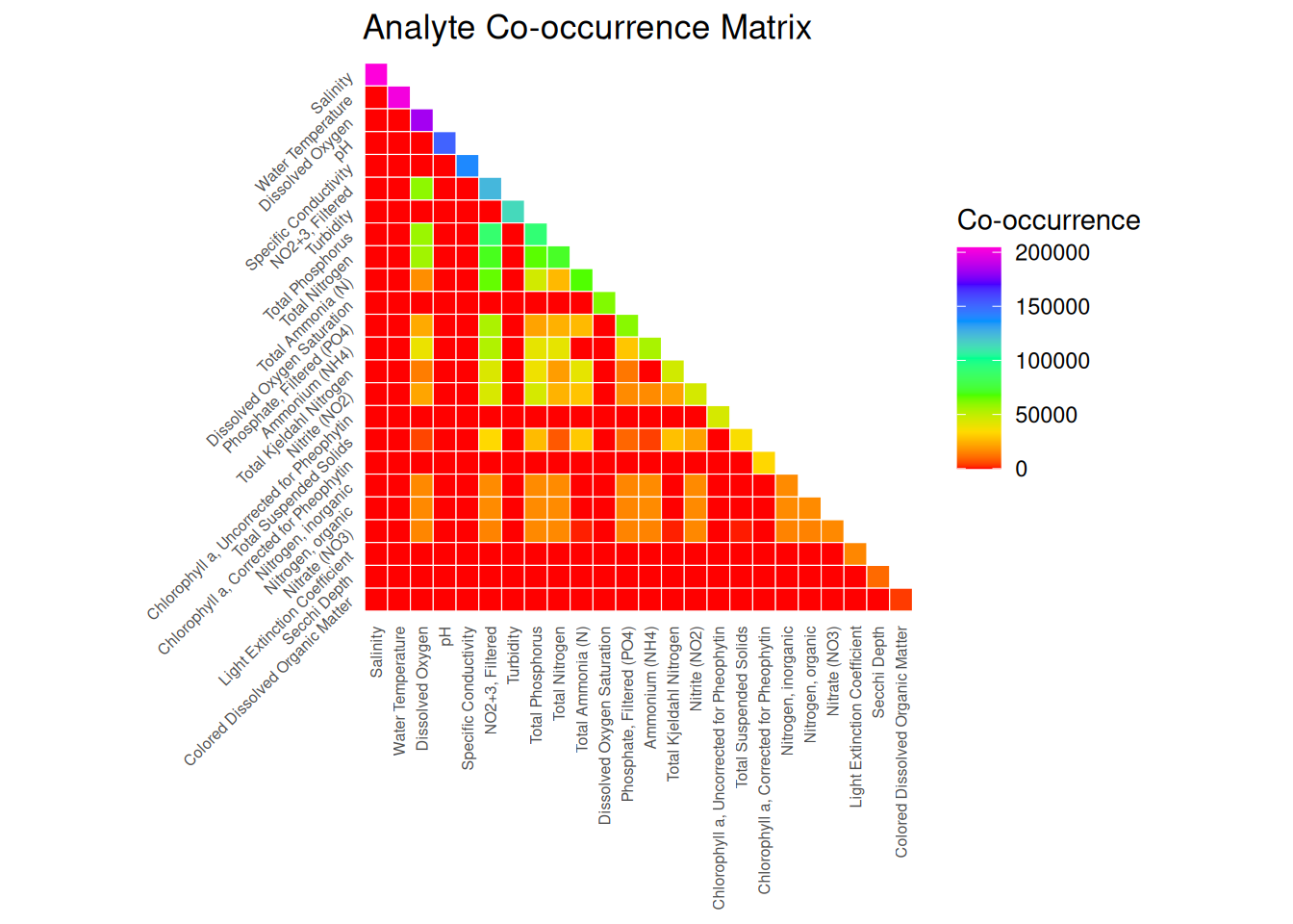
library(dplyr)
library(tidyr)
library(ggplot2)

# 1. compute analyte order (most -> least)
analyte_order <- df_wide %>%
  summarise(across(all_of(analyte_columns), ~ sum(!is.na(.)))) %>%
  pivot_longer(everything(), names_to = "Analyte", values_to = "Count") %>%
  arrange(desc(Count)) %>%
  pull(Analyte)

# 2. presence matrix using sorted analytes
presence <- df_wide %>%
  mutate(across(all_of(analyte_order),
                ~ !is.na(suppressWarnings(as.numeric(.))))) %>%
  select(all_of(analyte_order))

# 3. co-occurrence matrix (rows/cols are in analyte_order)
cooccurrence_matrix <- t(presence) %*% as.matrix(presence)

# 4. tidy it and set factor levels explicitly
cooccurrence_df <- as.data.frame(cooccurrence_matrix) %>%
  mutate(Analyte1 = row.names(.)) %>%
  pivot_longer(-Analyte1,
               names_to = "Analyte2",
               values_to = "Cooccurrence") %>%
  mutate(
    Analyte1 = factor(Analyte1, levels = analyte_order),
    Analyte2 = factor(Analyte2, levels = analyte_order)
  ) %>%
  # Keep only the lower triangle (row >= column)
  filter(as.numeric(Analyte1) <= as.numeric(Analyte2))

# 5. plot with y-axis reversed
ggplot(cooccurrence_df, aes(x = Analyte1, y = Analyte2, fill = Cooccurrence)) +
  geom_tile(color = "white") +
  scale_fill_gradientn(colors = rainbow(7)) +
  scale_y_discrete(limits = rev(levels(cooccurrence_df$Analyte2))) +  # <-- reverse y-axis
  labs(
    title = "Analyte Co-occurrence Matrix",
    x = NULL,
    y = NULL,
    fill = "Co-occurrence"
  ) +
  coord_fixed() +
  theme_minimal() +
  theme(
    axis.text.x = element_text(angle = 90, size = 6, vjust = 0.5, hjust = 1),
    axis.text.y = element_text(angle = 45, size = 6, hjust = 1),
    panel.grid = element_blank()
  )

Export Wide Format Data

# Export the wide format data
write.csv(df_wide, here("data", "exports", "dashboardDataSEACAR_wide.csv"), row.names = FALSE)

cat("Wide format data exported to: data/exports/dashboardDataSEACAR_wide.csv\n")

---

Note: Ideas for next steps: - Multivariate analysis where you need multiple parameters as separate variables - Creating correlation matrices between different analytes - Machine learning tasks that expect features as columns - Quick comparison of multiple parameters at the same observation point